
This article presents a simple experiment to illustrate how phase noise [1] converts to time-interval error (TIE) jitter [2]. This is of particular interest to hardware professionals who work with both jitter and phase noise, such as engineers analyzing reference clocks for high-speed SERDES, or sampling clocks for data converter, applications. Insight gained from this article can be used when debugging systems to identify and reduce various sources of timing noise.
One key difference between TIE jitter and phase noise is the type of noise processes observed by each [3]. To clarify this, Equation 1 represents an output voltage signal (Vout) as a baseband noise (B) plus a sine wave signal at a specific carrier frequency (ωc) that includes amplitude (A) and phase (ϕ) modulation noise.
Vout(t) = B(t) + A(t)×sin(ωct+ϕ(t)) Eq. 1
All three noise processes (e.g. A, B, ϕ) impact TIE jitter as measured by an oscilloscope. However, only phase modulation (e.g. ϕ) impacts phase noise when measured using a phase-noise analyzer (PNA, such as Keysight Technologies E5052B), since the PNA rejects amplitude noise during the measurement [3].
The process by which phase noise converts to TIE jitter is simply aliasing [4]. To illustrate this, we'll analyze timing noise in a phase modulated (PM) [5] sine wave clock carrier signal (e.g. sin(ωct)) appearing at the output of a signal generator. The PM signal in this experiment is also a sine wave (e.g. ϕ(t)=K×sin(ωpt)), whose frequency (ωp) is swept over some range. For example, Figure 1 shows a phase noise plot for a 100 MHz clock signal with added 1 MHz PM at roughly -40 dBc. Phase noise, as illustrated in Figure 1, is the spectral energy density of phase fluctuations in a signal. Incidentally, Figure 1 shows that the signal generator also outputs a much smaller spur of -86 dBc at 180 kHz offset frequency, which we'll ignore for the purpose of this experiment.
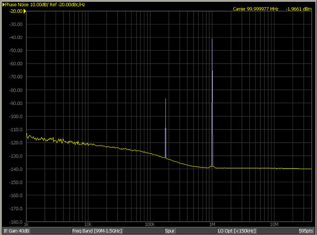
Figure 1 Phase noise plot of a 100 MHz clock signal with added 1 MHz PM at approximately -40 dBc.
Figure 2a illustrates the test setup, where the magnitude and frequency of PM on the 100 MHz carrier signal is quantified independently using (1) a real-time oscilloscope, (2) a dedicated PNA, and (3) a spectrum analyzer [3,6].
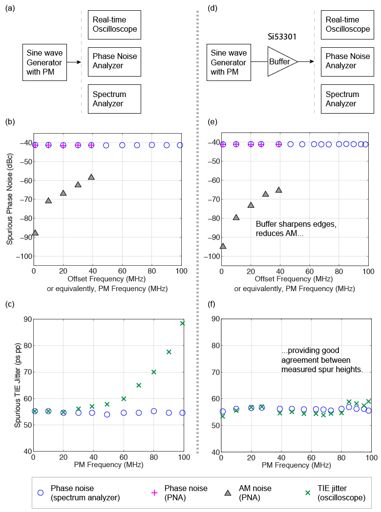
Figure 2 Experimental setup (a) for quantifying spurious PM in a signal as (b) phase noise and (c) TIE jitter. Illustrations (d-f) buffer the analyzed signal to remove AM noise, but are otherwise similar to (a-c).
The PM quantified as spurious phase noise is graphed in Figure 2b as a function of offset frequency. For example, the first phase-noise data point represents 1 MHz PM (e.g. ωp) on a 100 MHz carrier (e.g. ωc). Here, the offset frequency (x-axis) is equivalent to the frequency of the PM sine wave. The magnitude of PM (e.g. K) is adjusted to be relatively constant around -40 dBc, and the spurious data measured from the PNA (limited to 40 MHz offsets) agrees well with that from the spectrum analyzer, which extends to higher offset frequencies. For reference, amplitude noise (e.g. A) [7] is also measured using the PNA up to a 40 MHz offset frequency, and graphed in Figure 2b.
Figure 2c quantifies the PM as spurious TIE jitter and plots it versus PM frequency, which, in Figure 2c, is equivalent to the TIE jitter frequency. For reference, the spectrum analyzer data plotted in Figure 2b in units of dBc (which we'll denote as spurdBc) is converted to units of seconds peak-peak using Equation 2 [8].
Figure 2c shows that the spurious TIE jitter agrees well with the spurious phase noise for low PM frequencies, but increases exponentially above 30 MHz PM.
The reason for this increase in AM noise at the output of the signal generator is not relevant to our discussion, except in-so-much as to find a way to minimize the influence of this AM noise on measurements of TIE and phase noise. Recall that our goal is to understand how phase noise converts to TIE jitter, so the presence of amplitude noise in the signal may lead to false conclusions (since amplitude noise influences TIE jitter but not phase noise). Figure 3 illustrates the amplitude-to-jitter conversion process for 1 MHz and 99 MHz PM scenarios, where AM is clearly seen in the output signal for 99 MHz PM but not 1 MHz PM.
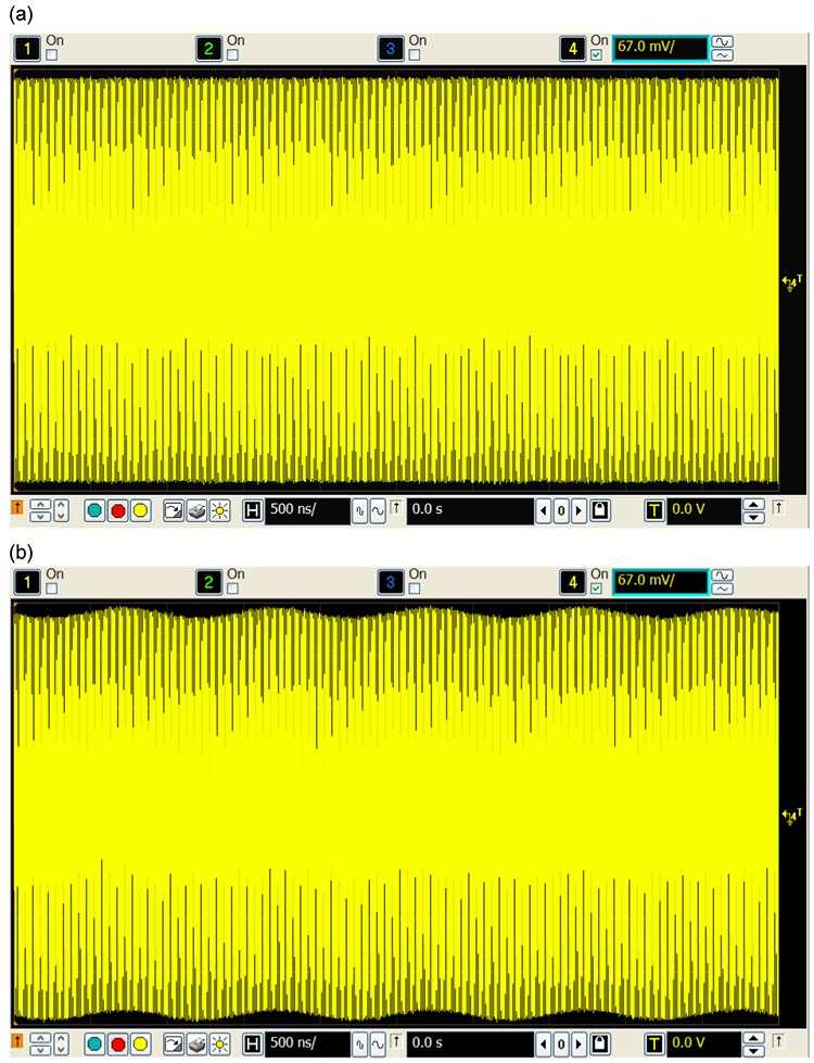
Figure 3 Output voltage waveforms corresponding to PM frequencies of (a) 1 MHz and (b) to 99 MHz, where the latter exhibits significantly higher AM noise.
Since we want to analyze how phase noise (alone) converts to TIE jitter, we need to first remove, or at least minimize, AM noise in the signal under test. We do this by buffering the signal as shown in Figure 2d, which reduces AM by 6 dBc as shown in Figure 2e. The buffered signal then shows good agreement between spurious magnitude measured with an oscilloscope versus spectrum analyzer as shown in Figure 2f. We therefore conclude that the magnitude of spurious PM (e.g. spur height, K) observed in a phase noise plot is preserved (except for a change in units from dBc to seconds peak-peak) when measured as spurious TIE jitter using an oscilloscope.
Having understood how the magnitude of phase noise maps to TIE jitter, let's analyze how its frequency translates. Figure 4 illustrates the aliasing process that occurs. The TIE jitter spectrum for rising clock edges on a 100 MHz clock carrier signal extends up to 50 MHz, which is the Nyquist frequency [9], as shown in Figure 4a. Thus, noise frequencies above 50 MHz will alias below 50 MHz when TIE jitter is measured. Phase noise, however, is measured offset from the carrier frequency, and so extends from 100 MHz to 200 MHz in the signal spectrum for this experiment, as shown in Figure 4a. The PM frequency is also offset from the carrier, and a separate scale is drawn along the top of Figure 4a to illustrate the sine wave frequency used to modulate the carrier. To simplify the discussion, each consecutive 50 MHz region in the signal spectrum is referred to as a "Nyquist zone" (NZ), where NZ #1 extends from 0 to 50 MHz, NZ #2 extends from 50 to 100 MHz, and so on for higher zones.
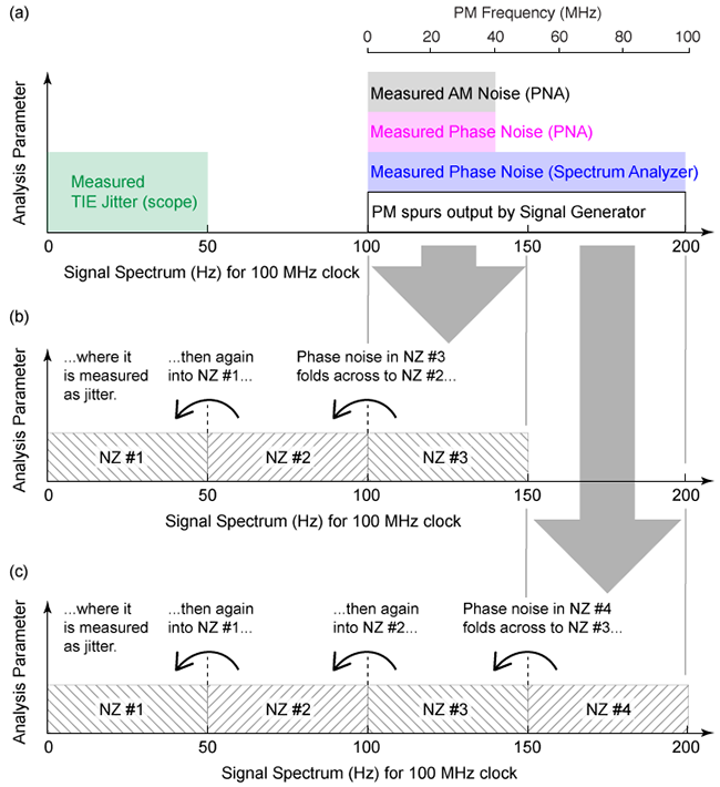
Figure 4 Phase noise measured in (a) Nyquist zones 3 and 4 alias to Nyquist zone 1 as illustrated in (b) and (c), respectively.
Spurious phase noise created by PM in NZ #3 and NZ #4 alias down to NZ #1 as shown in Figure 4b and Figure 4c, respectively. For example, spurious phase noise at 140 MHz reflects across 100 MHz to alias to 60 MHz, then reflects again across 50 MHz to alias at 40 MHz. Likewise, spurious phase noise at 199 MHz aliases to 101 MHz, which aliases to 99 MHz, which aliases to 1 MHz. Note that this last example describes the scenario illustrated in Figure 3b, where the 99 MHz PM tone includes significant AM, easily observed as a 1 MHz voltage envelope in Figure 3b.
Figure 5 uses multiple x-axes to map various frequency domains of interest in this experiment. The first x-axis shows how the PM frequency, which is offset from the carrier frequency, appears in the rising-edge TIE jitter spectrum (y-axis). Specifically, PM frequencies falling between 0 and 50 MHz appear in the signal spectrum between 100 and 150 MHz (i.e. NZ #3), and alias into the TIE jitter spectrum at the same PM frequencies, as illustrated in the left half of Figure 5. Similarly, PM frequencies between 50 and 100 MHz appear in the signal spectrum between 150 and 200 MHz, and alias into the TIE jitter spectrum at their mirror-image frequencies, as illustrated in the right half of Figure 5.
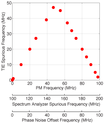
Figure 5 Frequency-mapping between TIE jitter and phase noise, illustrated via spurious PM on a 100 MHz carrier, showing that phase noise aliases to become TIE jitter.
Conclusion
This article showed that data in a phase noise plot, which is plotted offset from the carrier frequency, simply aliases into a TIE jitter spectrum. That is, higher-frequency phase noise aliases below the Nyquist frequency of a TIE jitter spectrum. The Nyquist frequency for a TIE jitter spectrum computed from rising (or, separately, falling) edges equals half the fundamental clock frequency. Alternatively, the Nyquist frequency for a TIE jitter spectrum computed from all clock edges equals the fundamental clock frequency (not discussed above). Finally, although the above experiment discusses only spurious phase noise, the conclusions apply equally to random phase noise.
References
[1] https://en.wikipedia.org/wiki/Phase_noise
[2] "Jitter Analysis," Application Note 5991-4000, Keysight Technologies (2014), http://literature.cdn.keysight.com/litweb/pdf/5991-4000EN.pdf
[3] "Influence of Noise Processes on Jitter and Phase Noise Measurements," G. Giust, Signal Integrity Journal (April 10, 2018), https://www.signalintegrityjournal.com/articles/800-influence-of-noise-processes-on-jitter-and-phase-noise-measurements
[4] https://en.wikipedia.org/wiki/Aliasing
[5] https://en.wikipedia.org/wiki/Phase_modulation
[6] "Phase Noise Measurement Solutions," Application Note 5990-5729, Keysight Technologies (2018), http://literature.cdn.keysight.com/litweb/pdf/5990-5729EN.pdf
[7] https://en.wikipedia.org/wiki/Amplitude_modulation
[8] "User Guide for Desktop Phase-noise Calculator," JitterLabs website (December 6 2016), https://www.jitterlabs.com/support/documentation/guide1.
[9] https://en.wikipedia.org/wiki/Nyquist_frequency