
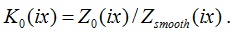
Metal loss is an increasingly important factor affecting design quality in all high-speed applications. As operational frequencies went up, it became evident that formulas ignoring roughness of the metal surface greatly underestimated losses. A number of approaches have been proposed over the years [1-3] that introduced additional losses by applying frequency-dependent correction to the impedance of the smooth metal. A recent survey in this area can be found in [4].
As of today, a widely accepted approach to model an impedance of the rough metal is taking a complex frequency-dependent impedance of the smooth metal and applying to it a multiplier  that monotonically grows from 1 to
  >1. Virtually all publications on this topic (and a vast majority of commercially available simulators) assume that this correcting multiplier is a real-value function. In the literature, it is often called “roughness correction factor.”
Since the internal impedance of the smooth surface is described by the well-known “skin effect” formula, where real and imaginary parts of the impedance are equal, applying a real multiplier to it obviously produces the complex value where the parts (resistive and inductive components of impedance) are also equal. For example, [2-4] give us the following relations:, 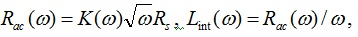 making
  and
and  definitely equal. Similar equations/statements can be found in many other publications, including major textbooks.
Is this a physically valid model of metal impedance? Can we apply a frequency-dependent real multiplier to a causal dependence, which the smooth impedance formula definitely is, without violating causality? There are only few sources known to us that have raised these questions.
First, this issue was addressed in [5] where the authors mention that inductive and resistive portion of the metal’s internal impedance are generally not equal, but should be mutually related by Hilbert transform to enforce model causality. Indeed, the roughness correction factor  was defined and derived as a ratio of the active power dissipated on a rough metal to that dissipated on a perfectly smooth metal. From here, it follows that it describes proportionality between the resistive portions of the impedance only. As to wording, it would make sense to call
  a “loss correction factor” because we have no evident reasons to believe that inductive component should be increased in the same proportion. Another publication [6] actually applied this idea to find a causal version of Huray’s roughness formula.
It’s remarkable that these results, despite laying a perfect ground for building physically meaningful causal models of metal roughness, went majorly unnoticed. Hence the commonly used practice hasn’t changed since then. Perhaps, this can be explained by the fact that [5] did not provide practical examples of causal versions of known models, while [6] might appear too academic to the readers, and possibly didn’t contain enough evidence that would convince them to immediately start using the causal model.
A far-reaching goal of this paper is to give an additional impetus to this development and make causal roughness models part of the mainstream paradigm when simulating metal losses. As we remember, this happened a few years ago with the introduction of causal dielectric loss modeling [7, 8]. Now is the time for the metal.
In addition, we would like to fill in some knowledge gaps regarding this subject, such as:
- General approach to derivation of causal models from given analytical expression (or another reasonably complete description) of the metal loss correction factor.
- Basic relationships existing between loss correction factor, inductance correction factor, complex correction factor, real and imaginary parts of internal impedance and inductance of the rough metal.
- Side-by-side comparison of those dependences between causal and non-causal versions of Hammerstad and Cannonball-Huray models.
- Derivation of causal roughness model from loss correction factor specified as tabulated dependence.
We also show that:
- As necessitated by causality requirements, inductive portion of the internal metal impedance of the rough metal is not equal, but appears much larger than the corresponding resistive portion of it.
- We analyze the effect of using a causal model of metal roughness on the characteristics of transmission lines. Under other conditions being equal, a causal model makes the line’s delay and characteristic impedance larger than with non-causal models. We provide expressions which formally evaluate this difference.
- We compare measured characteristics of stripline to simulations when using causal and non-causal versions of the Cannonball-Huray roughness model [11]. The Cannonball-Huray model is a simple model, based on cubic close-packing of equal spheres, which can be used to determine the sphere radius and area parameters for the Huray roughness formula. The cannonball stack is an example of a cubic close-packing of equal spheres, thus the name for the model. By obtaining published conductor roughness parameters, solely from manufacturers’ data sheets, the model has shown excellent agreement to measured results up to 50 GHz.
This paper is organized as follows: Section I gives general relationships for the causal roughness correction multiplier, and outlines the process of deriving a causal correction factor for a given analytical expression for the loss correction coefficient. In Section II we apply this approach to Cannonball-Huray and Hammerstad models. Section III analyzes the results for Cannonball-Huray and Hammerstad models. In Section IV, we evaluate the effect of using causal models when analyzing lossy transmission lines. In Section V we outline the process of finding a complex causal model when the loss correction factor is given by a table. In Section VI, we describe the Cannonball-Huray roughness model in more detail. Then, we validate the model, through a case study, using causal and non-causal versions of Cannonball-Huray formula and compare them to the measured results.
I. General relationships
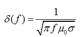
As shown in [2, 3], an internal impedance of the metal with smooth surface is related to the skin depth, an effective penetration of electromagnetic field into metal surface:
 (1)
(1)
where  is frequency (Hz),
  is permeability of free space (H/m) and
  is metal conductivity (S/m). As follows from this formula, the thickness of the effective conducting layer decreases as
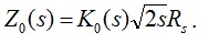
  , thus causing an increase in metal impedance in inverse proportion. From here it follows a well-known formula for the complex impedance of the smooth conductor:
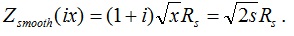
 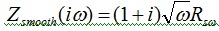 , which we will slightly modify and represent as a function of the normalized frequency x :
 (2)
(2)
Here Rs is a “skin resistance,” a constant factor that absorbs some material and geometrical parameters of the conductor, and s = ix is a complex frequency. It is convenient to establish proportionality between the normalized frequency x and the angular frequency  individually for each type of metal roughness model, and we will select it later. An impedance of the rough metal surface, under other conditions being equal, is larger and therefore can be expressed as
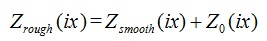 (3)
(3)
where  is an additional impedance due to metal roughness. As stated in [5], total and additional impedance caused by metal roughness must be a causal function, so that
  and
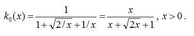
and  must be mutual Hilbert transforms. In [1] and in many other sources, the loss correction factor is defined as a ratio of the power dissipated in a rough metal to that dissipated in a perfectly smooth metal. From this definition it follows that loss correction factor
  , a real function of frequency, is also the ratio of the resistive part of impedance of rough metal to the resistive part of impedance of smooth metal:
 (4)
(4)
In all practical cases it is assumed that  , because metal roughness makes no addition to impedance at low frequency.
Note that it would be improper to use the relations 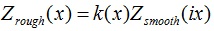 or
or 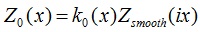 , because we have no evidence that roughness modifies inductive (imaginary) part of impedance in the same proportion as it does for resistive (real) part. Instead, we should assume that there exists similar relationship with complex (yet unknown) factor
  :
:
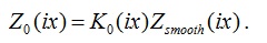 (5)
(5)
How can we practically find  ? From (2) and (4), it follows that:
 (6)
(6)
and we also know that  must be a causal function. For causal complex function, the imaginary part can be restored from the known real part (6), by using certain types of Kronig-Kramers (K-K) relations. Once the missing imaginary part
  is restored, the unknown complex correction factor can be found as:
 (7)
(7)
With a known causal complex correction factor, an additional impedance due to metal roughness becomes:
 (8)
(8)
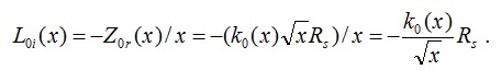
From (8), we can express the factors at real and imaginary parts of the impedance of smooth metal as:
 (9)
(9)
As we see, real and imaginary parts of skin impedance are increased by different factors. The one in the real part describes loss correction factor, the other is an inductance correction factor. Also, comparing (4) and (9), we see that
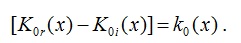 (10)
(10)
This result matches [6]. An important conclusion from here is that for a given complex correction factor that applies to complex impedance of the smooth metal, the loss correction factor is a difference between its real and imaginary parts; whereas, an inductance correction factor is a sum of real and imaginary parts of the same complex factor. As we see, metal roughness modifies resistive and inductive parts of the smooth metal in different proportion.
Below, we will also need an expression for an additional complex inductance caused by metal roughness. It can be found as a ratio of the complex impedance (8) and complex frequency as 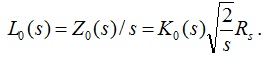 Real and imaginary parts of the complex impedance and inductance are related as
  . Therefore, imaginary part of the inductance can be found as
 (11)
(11)
As we see, it is fully defined by the loss correction factor.
II. Finding causal correction factor for Cannonball-Huray and Hammerstad models
Cannonball-Huray model
We will use the above equations to illustrate the process of deriving a complex correction factor for a single component of the Cannonball-Huray roughness model. As shown in [3, 11], these models define loss correction factor in a form of the sum
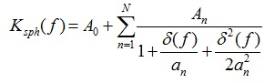 (12)
(12)
where δ(f) is a skin depth defined in (1), an are radii of spherical shapes representing rough metal, and factors An are constant and defined by geometry assumed by each model.
Let’s consider n-th summand in (12), assuming An = 1. By introducing a dimensionless normalized frequency 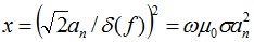 , we represent this component as a simple function of a single argument:
 (13)
(13)
Then, using definitions and ideas from Section I, we derive a complex factor as shown in Appendix A. This factor becomes 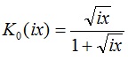 . Considering all summands in (12), the final result becomes:
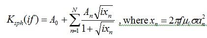 (14)
(14)
Hammerstad model
Hammerstad loss correction factor [2] is given by equation:
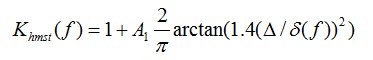 (15)
(15)
where  is RMS surface roughness, and
  is skin depth. The normalized offset-free factor here is
 (16)
(16)
Derivation of the complex correction factor can be found in Appendix B. The resulted causal factor becomes:
 (17)
(17)
where s = ix is complex frequency, and x is defined in (16).
III. Causal versions of Hammerstad and Cannonball-Huray roughness models
The approach we outlined in the previous section can be applied to any other model type, if the loss correction factor is represented by a continuous analytical function. Some details could be different though, such as variable techniques when finding K-K integral.
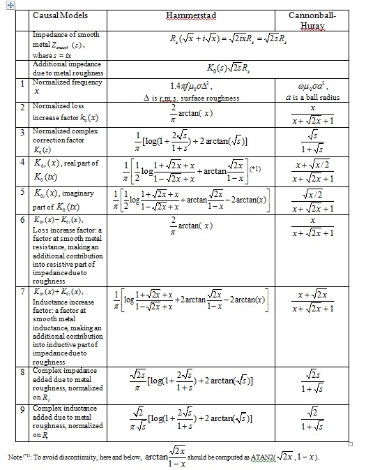
In this section we present formal results for causal and non-causal versions of Hammerstad and Cannonball-Huray models. To allow side-by-side comparison, we put formulas into Table 1 below. For completeness, the table contains the definition of smooth metal impedance and the normalized frequencies used in each case.
As we see, complex characteristics, such as normalized complex correction factor, impedance and inductance added due to metal roughness, are functions in complex frequency. There exist inverse Laplace transforms of these characteristics, thus proving their causality. At the same time, these models provide loss increase factor (#2 in the Table 1), exactly as defined for the corresponding model types.
Table 1. Formulas describing causal Hammerstad and Cannonball-Huray models
Let us now analyze these results side-by-side. In the plots below, characteristics of the Hammerstad model are shown by dashed lines, while Cannonball-Huray model ones are shown by solid lines. If the plot provides real and imaginary parts of the dependence, they will be shown by red and blue color respectively. By [#n], we denote its position in Table 1.
In this section we intentionally consider the functions in normalized frequency, even though the exact definition of the normalized frequency in both cases is different. The functions may also have different multipliers. If the difference were only due to scaling/ normalization, it would be possible to overlap the curves on the logarithmic plots by shifting them along the axes. However, it is more than that, and we cannot make the curves coincide.
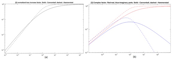
Figure 1. (a) Hammerstad and Cannonball-Huray loss correction factor [#2]; (b) real/imaginary parts of the complex correction factor [#4, #5]
The plots in Figure 1a are loss increase factors for the two models. Both have similar asymptotes, although the Hammerstad model demonstrates steeper transition from linear grow to steady region.
Figure 1b shows real and imaginary parts of the complex correction factor. It helps to better understand the differences in the models’ behavior. Real parts have similar asymptotes, at low and high frequencies, but imaginary parts do not. At low frequency, the real and imaginary parts grow as  , but at high frequency, the imaginary part decreases as
  for Cannonball-Huray, and
  for Hammerstad.
Limitations of the Hammerstad model become obvious when designers start to work at frequencies that correspond to the declining portion of the dependence. It turns out that the Hammerstad model settles too fast.
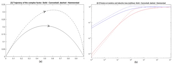
Figure 2. Trajectory plots representing complex factors [#3] over frequency range (a). Factors in resistive and inductive components of additional impedance, [#6] and [#7], (b)
Trajectories in Figure 2a illustrate the behavior of the complex correction factors over frequency. Note considerable asymmetry for the Hammerstad correction factor. It approaches saturation level much faster than Cannonball-Huray. The non-causal versions of both models, if plotted, would show a straight line segment along real axis, from 0 to 1.
Figure 2b shows multipliers (at skin impedance) creating additional resistive and inductive components due to roughness. Loss (resistive component) is defined by red curves [#6], the same as original real correction factors [#2] in Figure 1. Blue curves [#7] show the factors that apply to inductance. At low frequency, they grow as  and considerably exceed resistive, which grow as
  . A non-causal model would make both factors equal [#2] (red) thus causing considerable underestimation of internal inductance.
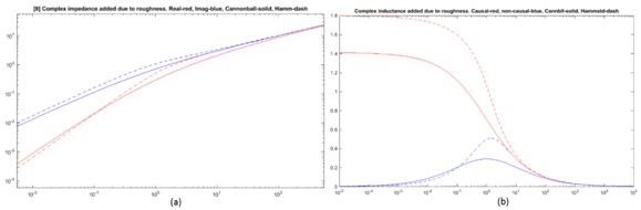
Figure 3. (a) Complex impedance contributed by metal roughness: resistive portion (red) and inductive (blue), [#8]. (b) An additional complex inductance, per [#9] in Table 1. For convenience, imaginary part of inductance is shown with opposite sign (as positive)
Figure 3a illustrates the complex impedance added due to metal roughness. The resistive portion is shown in red; inductive is shown in blue. In both cases, the inductive component considerably exceeds resistive. The non-causal version suggests that both are equal and coincide with red. Both models provide similar asymptotes at low and high frequency. At low frequency, the inductive part of impedance grows as , while the resistive part grows as  . At high frequency, they both grow as
  . However, Cannonball-Huray dependences are smoother (solid lines).
Figure 3b shows complex inductance added due to metal roughness. It is what we used in K-K relations. The real part of inductance is shown by red, while the imaginary part of inductance with opposite sign is shown in blue. Note that the negative imaginary part of inductance, after multiplication on complex frequency, becomes positive loss resistance. When using a non-causal model, both real inductance and loss would coincide with the blue curve, making inductance vanish at low frequency. To some extent, a dramatic deficiency of inductance in the non-causal model remained unnoticed, due to the fact that inductance doesn’t produce large impedance at low frequency. Still, as we will show, this difference is noticeable and practically important.
So far, we have only considered additional impedance caused by metal roughness. This impedance corresponds to  in equation (3). But how significant is this contribution when impedance of the smooth metal is factored in?
Let us analyze  , which is an internal impedance of rough metal that includes both components. Here, however, we need to know one more parameter. When studying addition to impedance due to roughness, we assumed that the loss factor k0 (x) in (4) is normalized, i.e.
  . Now, let’s consider
  with factors varied as A = 1,24,8.
The results are shown in Figure 4, (a)-(d). It is interesting that inductive and resistive components of the impedance in Figure 4 (a), (c) are not equal, and do not exactly behave as  . They do so only at very low and very high frequencies. But in the middle they have an inflection that happens at different frequencies for resistive and inductive components.
Also, as we can see in Figure 4 (b) and (d), even in the combined impedance, the ratio between the inductive and resistive component is considerable and reaches factor 2-3.
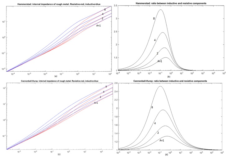
Figure 4. Skin impedance modified by roughness (left). Ratio of inductive component to resistive (right). First row corresponds to Hammerstad, second to Cannonball-Huray
IV. Causal roughness models and characteristics of transmission lines
If we want to know how model causality, or non-causality, affects the characteristics of transmission lines, we need to consider more variables and parameters. In this section, we assume that per-unit-length (PUL) parameters of the single-conductor transmission lines are known, and will evaluate the effect of using a causal model on a number of important characteristics, namely insertion loss, phase delay, and characteristic impedance. This way, we will get general estimates of the error in a formal way.
We start from the line’s propagation operator, and will try to simplify it, assuming that the resistive loss produces a smaller contribution than the inductive portion of impedance. Similarly, assume that dielectric loss produces a smaller conductance than that of the capacitance.
Therefore, the losses can be separated in the propagation operator as follows:
 (18)
(18)
In (18) we assume that metal and dielectric losses,  respectively, are purely real because the corresponding imaginary parts are absorbed by frequency-dependent PUL inductance and capacitance
  . For brevity, we will omit frequency arguments in these variables.
Thus, imaginary and real components in the power can be separated as follows:
 (19)
(19)
Magnitude of the propagation operator in (19) can be converted into insertion loss:
 (20)
(20)
If there is a loss correction factor in  , it should be visible on the insertion loss plot as a multiplier to the skin resistance. As implied by #6 and #7 in Table 1, the resistive part has a multiplier
  , whereas the corresponding contribution into an inductance gets the multiplier equal
  . From here, we can represent frequency dependent inductance as
  , where
  is a value of inductance at “infinity.”
A non-causal roughness model applies an identical factor to both resistive and inductive contributions from skin impedance. That is, the resistive losses are similar to causal case, but inductive component 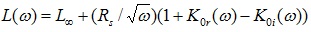 is smaller because
  . For convenience, we denote the common part of inductance that presents in both cases as
  . Then, inductance for causal and non-causal cases becomes
  respectively.
Is the magnitude of the propagation operator affected by non-causality?
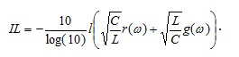
When computing insertion loss in (20), resistive loss is the same, regardless of model causality. What changes is inductance. It becomes larger when using a causal model. Larger inductance will reduce the effect of resistive losses and increase conductive losses. However, resistive losses dominate at low frequency, and conductive ones at high frequency. That’s why the model with causal roughness will show slightly less loss at low frequency but larger at high frequency. The variation of insertion loss can be estimated as:
 (21)
(21)
The difference is very small because the multiplier changes its sign and remains close to zero.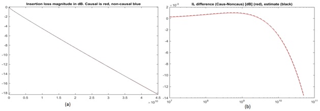
Figure 5. (a) IL plots for causal and non-causal models (red/blue), (b) the difference between IL dependencies: red – found directly from the extracted S-parameters, dashed blue – estimated.
In Figure 5 a, b, we compare insertion loss from S-parameters generated with causal and non-causal roughness models. Figure 5a shows that IL plots are practically identical. The difference is indeed very small, as seen in Figure 5b, and the sign changes at approximately 3GHz. Formula (21) gives very accurate estimate, shown by dashed line.