
Editor's Note: This is a summary of a much longer treatment on this topic, which can be accessed at this PDF link.
In a perfect world, I’d like to be 6 ft. tall, smart, and handsome; unfortunately, as my wife can attest, I do not meet any of those conditions. The same happens with S-parameters in signal integrity. For the most part (not always) when we see a smooth curve, nicely behaved without ripples in the frequency domain we feel the world is safe. On the other hand, when we see weird resonant stuff or big dips/peaks in S-parameters, we are left wondering and asking ourselves: what is going on? (with a few adjectives in between).
Let’s take a quick look at Figure 1. I’ll venture to say the blue curve is a thing of beauty, but the red jagged curve is awful. As you might have guessed, the blue curve is a nice transmission line, the red curve is the same length line with some half-wave resonances superimposed on them. We’ll come back to this later.
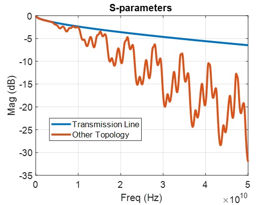
Figure 1:Transmission Line vs. Complex Topology S-parameter
Over the years I’ve come to realize that, particularly in signal integrity, half-wave resonances are often the cause of ugly S-parameters. You can argue that any type of resonance would cause problems, and you would be right. However, half-wave resonances are easily formed in topologies (as will become evident later), so let’s take a look at what conditions are necessary for them to develop.
Perhaps the easiest way to explain the condition necessary for a half-wave resonance to develop is through the illustration in Figure 2. Imagine two kids swinging a rope. Close to their hands, they will need to move the rope a little in order to excite it so that it swings up and down. In between the kids, right at the center, the rope will swing the most, reaching its peak. In this analogy, imagine the rope to be an envelope of any other oscillation that can occur, but never outside that envelope.
You immediately realize the rope has a shape that resembles half of a full waveform, or in other words, the full waveform will need a distance equal to two times the distance between the kids.
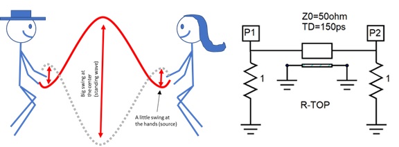
Figure 2: Half-Wave Resonance Fundamental
As you see in Figure 2, the circuit analogy is evident. We represent the distance between the kids as our transmission line. The fact the kids have a hand that almost doesn’t move, as the termination at each end, and the ports P1 and P2 as the source, or the force the kids are using to move the rope. You see, it does not matter how much the rope will want to swing at the kid hands, it will not be able to, since the kids are pulling it, holding it steady. At the center of the rope the situation is very different; the rope is free to move as much as it wants.
In summary, for a half-wave resonance to occur we need the following conditions to occur:
- Two terminations/discontinuities of the same kind (similar but not necessarily identical), separated by an electrical distance.
- A transmission line medium with some delay to separate the end terminations.
- Termination at both ends with different impedance from the transmission line characteristic impedance
 This allows us to call the end terminations discontinuities.
In the example above, the terminations are , and the transmission line characteristic impedance is
  . In other words,
  . It is important to understand that in circuits, half-wave resonances can be developed with exactly the opposite condition as well, meaning with
  . A similar half-wave resonance will occur but with maximum at the ends and minimum at the center.
Now that we know the conditions required for a half-wave resonance to develop I want to come back to a previous point made. Why are they so common in signal integrity topologies?
One way to imagine SI topologies generically is to think of them as some sort of uniform baseband transmission framework that is populated with different components (see Figure 3). Anything could constitute a component, from DC blocking caps to all kinds of connectors, cables etc. Usually when we attach these components to the baseband topology, the attachment at each end is approximately the same, producing similar discontinuities. If we consider that most elements/components have some sort of intrinsic delay or electrical length, we realize we perfectly meet the conditions for a half-wave resonance to occur and that is why, just the simple act of placing elements along interconnects promotes half-wave resonances.
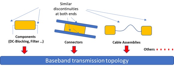
Figure 3: Topology Architecture
You might be quick to think: "If every single time I need to create a complex topology, I’ll have these pesky half-wave resonances, I am doomed!” Well, yes and no. As you might imagine, like everything in SI there are ways to minimize it, and the extent you’ll see these resonances will vary depending on several conditions. We will come back to this a bit later.
Let’s go back to Figure 1 and analyze the jagged line more. Figure 4 is the magnified version of this where we can identify two resonances. We see a lower frequency resonance  repetition, and a high frequency resonance
  repetition. ( I know, I am calling
  to a lower frequency than
  this is simply because we are computing a frequency in the frequency domain, meaning the x-axis is the frequency domain, so
  has less number of repetitions per unit than
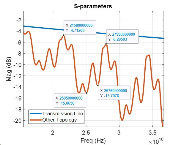
Figure 4: Mystery Topology with Dual Resonance
Let’s say we know the red curve represents a complex topology having a baseband per unit length propagation delay of  and by looking at the curve and all the resonances we suspect most likely it has several discontinuities. With that framework we would like to see if we can determine the separation between those discontinuities just by looking at the S-parameter insertion loss.
By recalling our jumping-rope kid example, we concluded the resonance formed is a half-wave resonance. (This means that the full wave would be two times the distance between the kids.) In the circuit world, we are going to replace the word distance by electrical length, and mathematically we can convert the resonance frequency measured to distance as follows:  If we know approximately the transmission line propagation delay, that in our case is
  then just by simply looking at the frequency domain we can calculate the approximate length between discontinuities.
Let’s do that: 
In essence just by looking at the frequency domain S-parameters, if we assume we have only ½ wave resonances we could estimate there should be two sets of discontinuities, one set separated by  and another set separated by approximately
Figure 5 shows the mystery topology that produced the red curve shown before. As you can see this is a simplified behavioral topology with transmission lines with different lengths but with the same characteristic impedance of  and per unit length propagation delay of
  Also, the topology has lumped elements that could represent the attachment discontinuities for different components.
This topology is very simple just to illustrate the point, but please note the exact same behavior will happen on more complex topologies. For example, something very similar to the  piece with the two capacitors at the end will happen when you have a
  connector attached at both ends with vias not properly tuned.
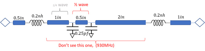
Figure 5:Mystery Topology Revealed
Ultimately just by analyzing the frequency domain, we were able to correctly identify the strongest of the resonances  The smaller
  resonance is coming from another type of resonance called a ¼ wave resonance and topic for a future article. We notice the interaction between the two inductors (same type of discontinuity) is not readily seen or it’s heavily masked and attenuated by the other bigger resonances.
The main point is that armed with this knowledge and using a very simple formula, we could attempt to track and minimize resonances.
But wait a second, so far, we have discussed how to identify half-wave resonances in our circuit which is part of the battle, but we have said nothing about how to minimize them.
Resonance Mitigation
There are two fundamental ways to minimize these resonances:
- Reduce the discontinuities magnitude (reflections at the ends)
- Increase the losses between discontinuities
To illustrate this point, I’ll cheat and use a 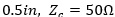 transmission line topology, but I’ll calculate the S-parameters with 40
 renormalization impedance as shown in Figure 6.
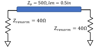
Figure 6: Simple Transmission Line with 40 Renormalization Impedance
Using a different renormalization impedance from the transmission line  creates in the simplest way the right condition for a ½ wave resonance to develop. Notice we end up with two terminations at the ends that are different than the transmission line characteristic impedance, creating two equal reflections at the ends and meeting the condition for a half-wave resonance to develop.
A deeper discussion of using S-parameter renormalization impedances to our advantage can be found in a previous article, “S-Parameter Renormalization, the Art of Cheating” [1].
As mentioned before, increasing losses would tend to minimize the effect of these resonances.
We can envision two ways to increase losses, either by changing the medium (such as by changing loss tangent) or by increasing the length of our  transmission line as shown in Figure 6.
And remember, changing losses by loss-tangent does not change the total delay from end to end of the transmission line, meaning the resonance period in the frequency domain will remain the same. On the other hand, changing the length of the transmission line, does change the overall delay from end to end, and hence the resonance period of the half-wave resonance will change.
Figure 7: Reducing Discontinuities by Increasing Losses: (Left) Increasing loss-tangent, (Right) Increasing length with tan d=0.002
As seen in Figure 7, when we increase losses by increasing loss tangent, the resonance frequency remains the same, but as the losses increase, the resonance is more dampened. On the other hand, when we add losses by increasing length and use very low dielectric loss, we see two effects: dampened attenuation and resonance frequency change as the separation between discontinuities increases.
When visually observing the right side of Figure 7  certainly appears to be a lower frequency than
  so why am I saying
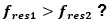
This is a common point of confusion for engineers. Please note we are measuring a frequency on a frequency axis, in essence it is the frequency of a frequency (this is called a Cepstrum) and that is why it is confusing. To unconfuse yourself, just measure the frequency value on consecutive peaks, and subtract. This has been shown previously in this article when referring to Figure 4 . When you do that, you’ll see that indeed  .
.
Let’s move on to the most obvious way to minimize these half-wave resonances.
We know to get a resonance we must have discontinuities that produce reflections at both ends, so the obvious way to minimize half-wave resonances is to minimize these discontinuities/reflections.
Figure 8: Resonance Amplitude Change by Impedance Magnitude
In Figure 8 we are using the same topology presented in Figure 6, and, by changing the S-parameters renormalization impedance  closer to
  , things keep getting better with smaller reflections.
Finally, when  there are no reflections and the half-wave resonance disappears.
This is a very simple way to show how the reflection’s magnitude affects the overall size of these half-wave resonances. This happens all the time in practical topological cases when the attachment of components is not properly designed, and the impedance of the attachment is very different than the impedance of the medium separating the attachment.
I believe it is important for the SI engineer to be able to fully understand, identify, and address these resonances in different topologies, so in addition to the short summary above, for the curious engineer and stout of heart, I have created a complete study of half-wave resonances in the frequency and time domain, with several practical examples and important derivations that can be accessed through this pdf link.
Reference
Blando, Gustavo. “S-Paraemter Renormalization, The Art of Cheating,” Signal Integrity Journal, 12 January 2017.