
Why does a low cost through-hole SMA have a lower bandwidth than a surface mount SMA? The answer will surprise you.
A coaxial connector is an electrical connector designed to work at frequencies in the multi-GHz range. Coaxial connectors are widely used in high-speed analog and digital applications. The family of coaxial connectors includes connectors such as the SMA, 2.92 mm, 2.4 mm, 1.85 mm, 1 mm, SMP(M), (M)MCX, BNC among others. These connectors are typically used with coaxial cables and are designed to maintain the impedance and shielding that the coaxial design offers.
A typical coaxial connector assembled on PCB can be divided roughly into two main parts: the cylindrical part on which the coax cable is screwed or pinned, and the part that is assembled to the PCB with the return path vias. The connector's bandwidth is limited by the first frequency that causes one of the connector's parts to resonate. At the resonance frequency, the wave impedance inside the connector increases dramatically, and so do the reflections from the connector.
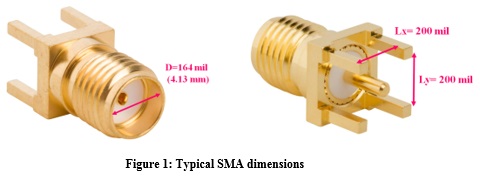
For example, in the sub-miniature version A connector (SMA) depicted in Figure 1 the cylindrical part of the connector has an outer diameter D=4.13 mm (164 mil) and it is filled with Teflon (εr=2.2). The part of the connector that is assembled to the PCB (dielectric constant is 3.8) is made up of four return path vias, which are 200 mil apart from each other.
As shown in Figure 2, as long as (1) Lx, Ly < λ (λ-wavelength), the structure with the four return path vias can be approximated as a closed structure with boundaries of highly conductive material that reflect the propagating waves and cause the structure to resonate at certain frequencies.
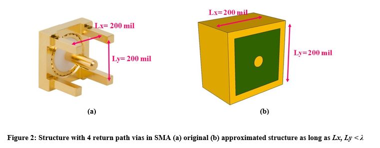
The structure in Figure 2 is a kind of rectangular cavity resonator. Assuming that the length of the return path vias is smaller than L =Lx, Ly, the possible resonance frequencies in this cavity is given by (2) [1]:
When (2) is identical for both TM and TE modes,  is the intrinsic propagation velocity and m,n are the mode numbers. As can be seen, (2) depends on the geometry (Lx, Ly) and the dielectric material (εr) of the cavity. However, not every fmn frequency will cause the structure to resonate. This depends also on the excitation itself: (a) whether the signal has energy at frequency fmn and (b) the location of the signal via inside the cavity. Different signal via locations will cause the structure to resonate at different fmn frequencies.
The first time that the structure in Figure 2 will resonate is when the length of its longest edge is equal to λ/2 (in this case assumption (1) is still valid). In our example, we obtain:
Figure 3 shows a simulation of transition through a signal via located in the middle of a structure with 4 return path vias.
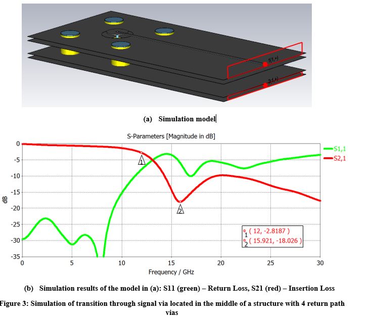
A number of observations can be made from the simulation results in Figure 3. The location of the signal via in the middle of the structure with four return path vias causes this structure to resonate at 15.9 GHz. A wide dip appears in the insertion loss at the resonance frequency, which degrades the insertion loss from 12 GHz and increases the return loss dramatically. Because the structure is relatively small (it cannot store significant energy) and the loss at 15.9 GHz is high, a low Q factor of 5.2 is obtained at the resonance frequency, which is expressed as a wide dip in the insertion loss. The next time the structure should resonate is when L=λ. However, in this case assumption (1) is not valid and, therefore, the structure with four return path vias cannot be analyzed as a cavity resonator. At frequencies above f10, the energy that the signal via radiates into the structure is no longer reflected back into the structure but leaks out of the structure into the PCB.
The other part of the coaxial connector (the cylindrical part) is a kind of circular cavity resonator. The possible resonance frequencies in this cavity for TM and TE modes are given by (4) [1]:
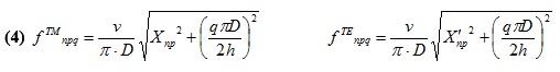
when n, p, q are the mode numbers. D and h are the diameter and the height of the cylinder respectively. X is the argument of the order n Bessel function of the first kind Jn(X), and X' is the argument of J'n. p is the order of the function when Jn(X)=0 or J'n(X')=0.
In order to find the first resonance frequencies for TM and TE modes, we determine q=0 . The smallest Xnp is X01=2.405, and the smallest X'np is X'11=1.841. In this case, we obtain the simple formulas in (5):

Substituting the dimensions from the example into (5) yields the first 2 possible circular mode resonance frequencies:
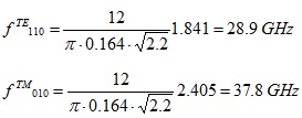
Figure 4 shows TM010 and TE110 electric and magnetic fields inside the cylindrical part.
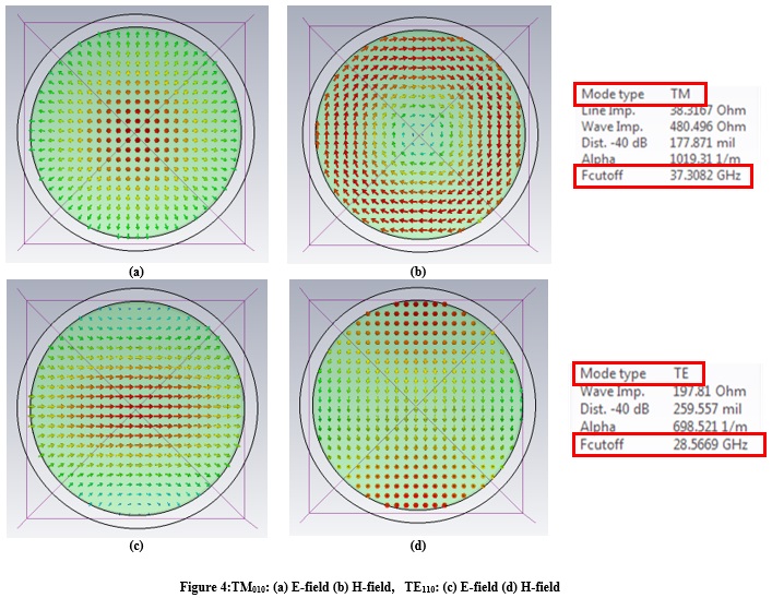
Because both f TE110 and f TM010 are larger than f10, we conclude that the rectangular cavity resonator, made by the four return path vias, determines the SMA bandwidth – and not the cylindrical part of the connector.
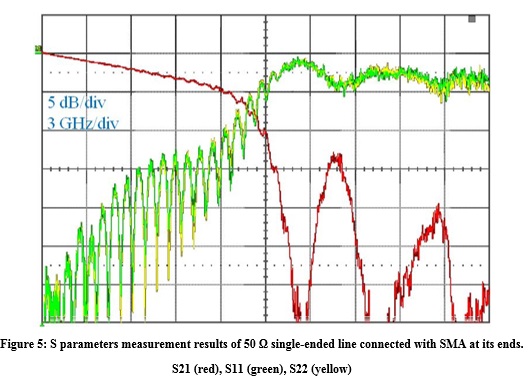
Figure 5 shows measurement results of a 50 Ω single-ended line connected with an SMA at its ends. The measurement results show the influence of the rectangular cavity resonator made by the 4 return path vias. A wide dip appears in the insertion loss at the resonance frequency (f10) at 16.5 GHz, which degrades the insertion loss from 12 GHz and increases the return loss dramatically.
In order to increase the SMA bandwidth, it is essential to change the return path via structure. Such a change can be seen in the optimized SMA design in Figure 6. In this design, the cylindrical part remains the same as in the SMA, but the return path via structure has been changed from rectangular to a smaller diameter, circular pattern.
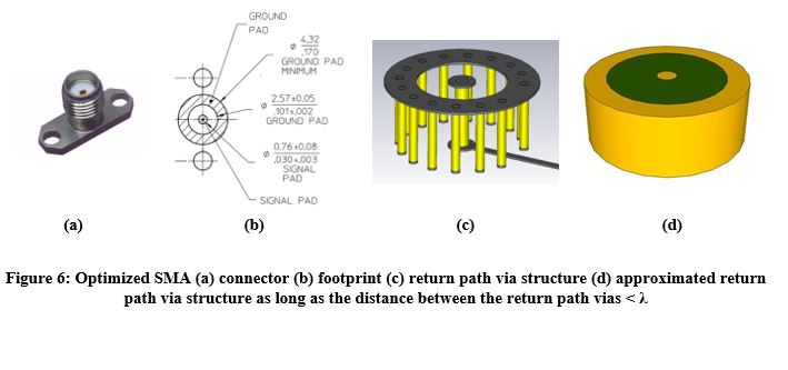
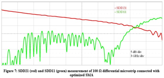
As long as the distance between the return path vias is smaller than the wavelength, the new return path via structure can be approximated as a cylinder with highly conductive material boundaries filled with the PCB dielectric as depicted in Figure 6(d). This structure is a kind of circular cavity resonator with resonance frequencies as in (4) and (5). For example, if we place the return path vias 50 mil from the signal via (D=100 mil), we obtain f TE110 = 36.1 GHz by using (5), which is more than two times f10. Another advantage of the cylindrical return path via structure is that it reduces significantly the signal via radiation into the PCB. Figure 7 shows the insertion and return loss measurement of a 100 Ω differential microstrip connected with optimized SMA. It can be seen that the insertion loss drops off monotonically with no resonances up to 24 GHz and with return loss less than ‑13 dB.
Further improvements in coaxial connectors are based on (5). According to (5), in order to increase the circular cavity resonance frequencies it is necessary to (a) reduce the dielectric constant inside the cavity, and, therefore, the Teflon (εr=2.2) is replaced with air (εr=1) and (b) to decrease the outer diameter D. These new coaxial connectors are named according to their outer diameter D: 2.92 mm, 2.4 mm, 1.85 mm, and 1 mm.
References
[1] R. F. Harrington, Time-Harmonic Electromagnetic Fields, Hoboken, New Jersey: Wiley-IEEE Press, 2001.