I use a function generator as a source to stimulate circuits and measure their response. I happened to have three different sine wave generators available with a price range of $12, $275 and $1200. I wondered just how much better the sine wave is from the more expensive function generator compared to the lower cost units. Just how much bang do you get for your buck?

Measuring Three Different Function Generators

Using my scope, I was able to compare these three sine-wave sources and worked out a simple way of comparing each source to an ideal source. This method can be applied to any waveform.

The three sources I had available are shown in Figure 1. The low-cost unit is a common function generator from eBay for $12.   The mid-priced function generator is actually the waveform generator built into the Digilent Analog Discovery scope. The entire 2-channel scope with 2-channel function generator, costs only $275. The high-end function generator is a Teledyne LeCroy WaveStation, very similar to units from Keysight and other high-end vendors.

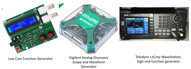
Figure 1. Three different function generators spanning in price from $12 to $1200.

The first step in characterizing the sine wave sources is to look at their voltage output on a scope. Figure 2 shows the measured signals when each was setup for a 50 kHz sine wave with amplitude of 1 V and no offset. The scope was set up to measure the signal from each generator, all on the same scale of 4 V full scale, 50 Ohm termination and the same time base of 50 usec full scale.

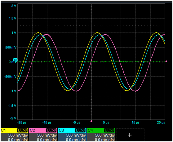
Figure 2. Measured sine waves from each source on a Teledyne LeCroy HDO8108 scope. The flat line is the voltage on channel 4 with no input, used as a reference to see the system noise level.

The vertical resolution of the scope is 12-bit. On this scale, the least significant bit (LSB) is 4 V/4095 = 0.98 mV. The time base was set for 125 Msamples/sec or a measurement every 8 nsec.

At first glance, they all look the same. This is when we can unleash the power of analysis tools to dissect the signals.

Second Step in the Analysis: FFT

The second step is to use an FFT. All modern scopes can take the measured data acquisition buffer and perform an FFT and show the signal in the frequency domain. I changed the time base scale to get a resolution of 100 Hz and a freq range of 1 MHz. It’s easy to reverse engineer my settings and know that I must have used a time base of about 10 msec and a sample rate higher than 2 Msamples/sec.  This is about 20,000 samples used to calculate the spectrum.

Figure 3 shows the comparison of the four spectra. In addition to measuring the three function generators, I also measured the noise on a channel with nothing connected. This is always a useful baseline when we are looking into the weeds at the fine details of signals.

An important best measurement practice is situational awareness- always be aware of the limitations of your instruments and how close your signal’s figures of merit are to the instrument’s limits.

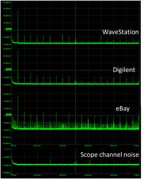
Figure 3. Calculated spectrum for the three sources and the channel noise.

The WaveStation and Digilent generators show very similar harmonic distortion. The first harmonic amplitude is about 60 dBmV, or 1 V amplitude, exactly as expected. The third harmonic is about -10 dBmV, or 0.3 mV amplitude. The even harmonics are lower.  These higher harmonics are more than 70 dB down from the first harmonic, but the harmonic distributions are slightly different.

The low-cost function generator has 30 dB larger harmonics and significant sub harmonics. Clearly the spectral quality is worse.

The scope baseline shows a similar noise floor of -40 dBmV, which is an equivalent amplitude of 10 uV. This is to be compared to the LSB of 1000 uV. To get this noise floor, we are effectively averaging over 20,000 measurements in the time domain. The expected reduction in noise is sqrt(20,000) = 141. The measured noise floor is about 1/100^th of the LSB noise, about what is expected.  There are only a few spurious peaks below the 100 uV peak level due to sampling frequencies in the ADC of the scope.

While this shows similar quality of harmonic distortion of the high end and my Digilent function generator, it is difficult to understand what the impact of this spectral distortion is on the original time domain signal. The question remains, how close are these real-world signals to “ideal” sine waves.

The way we can evaluate this question is by comparing the measured sine waves to simulated ideal sine waves.

The Collision of Two Worlds: The Ideal World and the Real World

All scopes allow exporting the measured voltage vs time data into a csv file. This csv file can be imported into a SPICE simulator and directly compared to an ideal sine wave to see the residual. Figure 4 shows the menu for saving each waveform. In this scope, I have six different formats from which to select. I used the Excel, csv format. After removing the text headers in this file it is exactly the format the simulator can read.

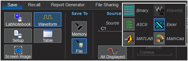
Figure 4. Six different formats of saving the voltage vs time data on a Teledyne LeCroy HDO8108 scope.

My favorite free version of SPICE is Quite Universal Circuit Simulator (QUCS). For an open source simulator, it is feature rich and easy to use.

I used a file-based voltage source to read the csv data from each channel of the scope. This is otherwise known as a piece-wise linear voltage source.

As a best analysis practice, it’s important to use exactly the same time step in the simulation as for which the data was measured. This way no interpolation is necessary.

This was an 8 nsec interval between measured or simulated points.

Each measured sine wave was brought into the QUCS simulation environment as a file-based voltage source. The voltage on the output node of the file-based voltage source was the measured voltage for each channel.

An ideal sine wave source was simulated to compare with the measured sine wave. An ideal sine wave has just three figures of merit, or parameters, that define it: the amplitude, frequency, and phase. I added a DC bias source to provide a fourth figure of merit to account for the real-world DC offsets in real waveforms.  These four terms were parameterized, so I could vary them until the simulated and measured sine waves gave the smallest residual difference. Figure 5 shows the circuit set up for one of the pairs of sine waves and the optimized parameters.

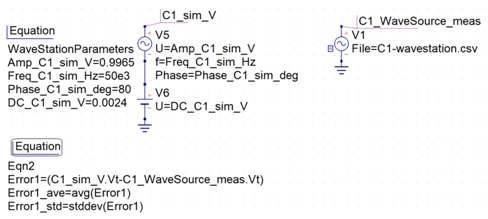
Figure 5. The simple circuit to compare a real measured waveform with a simulated ideal waveform and the parameters to set up the ideal sine wave. The residual error and some statistics were automatically calculated.

Using this simulation environment, I can collide the two worlds of the real measured sine wave with the ideal, simulated sine wave. I did this for each of the four waveforms, including the constant voltage reference channel. I optimized the four figures of merit for each sine wave to minimize the residual. What is left is the non-ideal error in each measured sine wave. These are summarized in Figure 6.

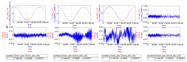
Figure 6. Top row: Comparing the measured sine waves and optimized ideal sine waves for the three function generator signals. Bottom series of graphs is the residuals. Note the LSB is about 0.001 V. The high and low LSB values are horizontal red lines.

The comparison shows what you get for the big bucks with a high-end function generator. The residual errors of the measured sine wave are just about comparable to the noise on channel 1, as seen in the far-right figure. The channel noise standard deviation is 2.03 mV, while the residual standard deviation between the ideal sine wave and the WaveStation is 2.56 mV, out of a 1 V amplitude.

The eBay function generator shows a much larger residual error than the mid-priced sine wave source.

This technique is a general method of evaluating how close to the ideal behavior any wave source is. If it can be described with an analytical function, the ideal waveform can be accurately calculated and compared to the measured waveform.

This is the same technique used to compare any real circuit with its ideal, simulated model. We measure the stimulus applied to the circuit and its response and compare these measurements to the simulated response. The residuals are a measure of the combination of the accuracy of our measurement system and the quality of the model.

This method is part of best analysis practices to gain confidence in our ability to accurately predict behaviors: we measure in the real world based on behaviors we simulate in the ideal world.