
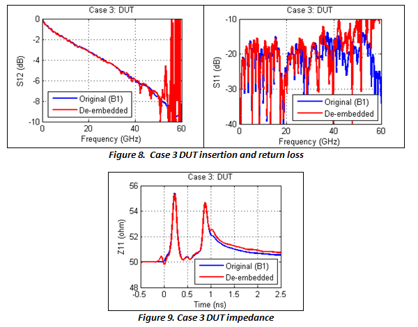
In case 3, the fixtures (A3+A4) are identical, and are ill-behaved. Vias exist in the paths of the fixtures as well as the 2x thru (B1), resulting in large reflections. The 2x thru's insertion loss (IL) and return loss (RL) cross each other at 13.2 and 33.7 GHz, as seen in Figure 7. Note that for good de-embedding results, RL should not exceed IL in general. After all, it is not possible to extract a DUT that is hidden behind a complete short or open. Under the special circumstance that the fixture and 2x thru are identical, as in this case, the DUT may still be extracted with good accuracy in the presence of strong reflections, as shown in Figures 8 and 9.
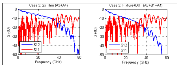
Figure 7. Case 3 insertion and return loss
In case 5, fixtures (A1+A2) are 50 Ohm microstrips and the 2x thru (A5+A6) is a 45 Ohm microstrip. The DUT, a 6 cm 50 Ohm microstrip (B1), is to be extracted. This setup was made to mimic the most practical applications where the fixtures and 2x thru do not have identical impedance at every location. The results, shown in Figures 10 to 12, demonstrate that the traditional 2x thru method (Dmbd-1) gives significant error in all IL, RL and TDR, while the impedance-corrected 2x thru method (Dmbd-2) is still able to extract the DUT with very high accuracy. The traditional 2x thru method splits the 2x thru directly for de-embedding, so the impedance difference between the fixtures and the 2x thru appear as non-causal error in the de-embedded DUT results. This non-causal error gives rise to artificial ripples in the DUT's IL and RL, and produces a response before time zero (and after the DUT) in the TDR waveform. The impedance-corrected 2x thru method, on the other hand, is free of causality error because it modifies the de-embedding S-parameters by matching the fixture's impedance.
Therefore, for the cases with noticeable impedance variation between the fixture and the 2X-thru structures, use of an impedance-corrected 2x-thru method is necessary to obtain good results.
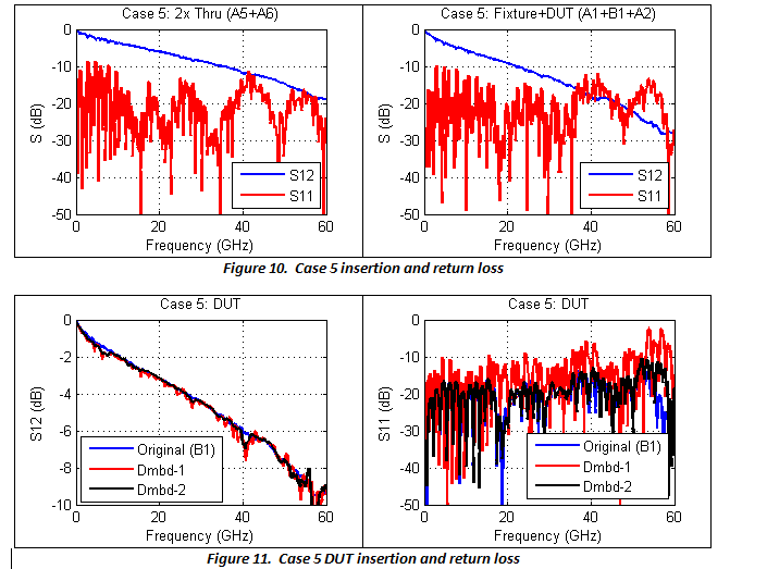
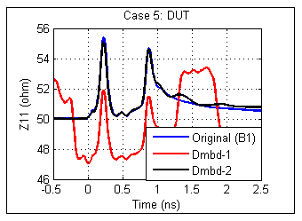
Figure 12. Case 5 DUT impedance
S-parameter Quality Tools and Metrics
Given the large amount of data typically contained in S-parameters, it is often difficult to ascertain the quality of the data without some quantitative evaluation. Manual comparison of plot traces is insufficient for quality assessment. Similar tools may already exist or will exist in the future, but the P370 committee also provides a free tool for all users to assess their own tool. Using DUT 5 as an example, application of the P370 quality tool to an S-parameter resulting from a suboptimal de-embedding algorithm produced the results shown in Figure 13a. The value of CQM in this case is 81 mV for a 10 Gbps data rate, a rather poor result. Note that the value is dependent upon the data rate, which determines the maximum frequency of interest. The corresponding value at 40 Gbps is 167 mV. The S-parameter that was extracted using the recommended 2x impedance corrected de-embedding algorithm, on the other hand, produced the results in Figure 13b, with a CQM value of 7 mV, a dramatically improved value.
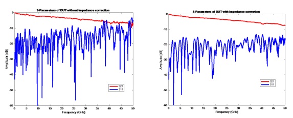
Figure 13. S-parameter plots for “bad” and “good” S-parameters
Figure 14 shows the s21 pulse response, indicating severely non-causal delay behavior for the suboptimal de-embedding case.
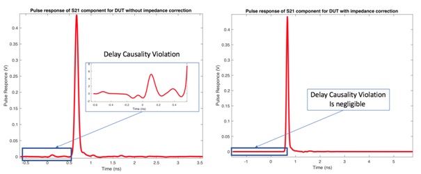
Figure 14. s21 Pulse response plots for bad” and “good” S-parameters
Table 2 summarizes the values of the three P370 quality metrics for these S-parameters. Both S-parameters are passive, indicated by the zero value for PQM. Severe non-causal behavior is found, as indicated by the 81 mV CQM value for the non-impedance corrected case. The non impedance-corrected data are only slightly non-reciprocal.
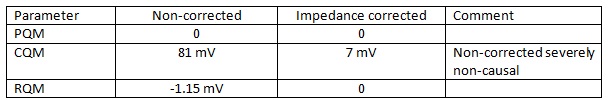
Table 2. Quality metric summary for DUT 5
Comparison of S-parameters
Quantitative comparison of S-parameters can be extremely useful in the validation of the data, and is more accurate than a simple qualitative (“eyeball”) comparison of plots of specific parameters; e. g., s21. A sample plot for one parameter (s11) for simulated and de-embedded results is shown in Figure 15. Figures 16 and 17 show the similarity metrics for two individual S-parameters from the same data. These would have to be reviewed for each individual S-parameter of concern; e. g., s11, s21, etc. Note that the port numbering in this example is not conventional, so s31 is the insertion loss.
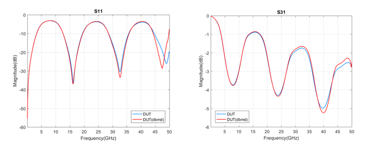
Figure 15. Measured and de-embedded s11 and s31 data comparison
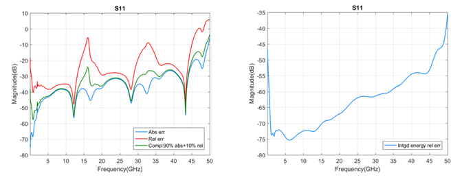
Figure 16. Sample s11 error plots and metrics
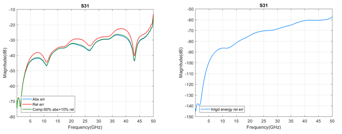
Figure 17. Sample s31 error plots and metrics
Conclusion
The IEEE P370 standard provides guidance on fixture designs, best practices, a data library for use in verifying de-embedding tools, and sample tools for evaluating and comparing S-parameter data. Designing fixtures and measuring devices for use up to 50 GHz is non-trivial, and it is hoped that this paper has given some insight into the potential use of the standard when it is published.
Acknowledgements
The authors would like to thank the members of the IEEE P370 committee for their contributions to the standard and this paper.
References
- Diepenbrock, J., et. al., “IEEE P370: A fixture design and data quality metric standard for interconnects up to 50 GHz,”.
This paper was originally presented at EDI CON USA 2018.