
As the digital data rates keep increasing, the bandwidth of the signals increases as well, and so does the attenuation of the interconnects. Therefore, the amplitude of the signals at the receivers becomes smaller, and in order to restore the data with a reasonable BER, it is necessary to keep the signal to noise ratio (SNR) as high as possible. Reducing various types of noise such as reflections, Mode-Conversion, Return-Path Bounce, and Crosstalk (Xtalk) becomes a serious challenge in signal integrity designs of high data-rate interfaces.
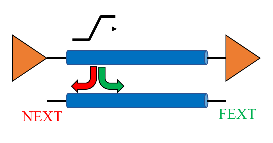
In practice, there are two types of Xtalk, as depicted in Figure 1. The first type is the Near-End Xtalk (NEXT), which is sometimes called backward Xtalk (or "coupling" in the analog RF world). The NEXT is the voltage measured on the victim terminated trace on the side close to the transmitter. The second type is the Far-End Xtalk (FEXT), which is sometimes called forward Xtalk (or "isolation" in the analog RF world). The FEXT is the voltage measured on the victim terminated trace on the side far from the transmitter. In this article, we will focus on the analysis and properties of the FEXT.
In general, every trace that carries an electrical signal (aggressor) has an electromagnetic (EM) field that distributes around it. The EM field amplitude decreases as the horizontal distance from the trace increases. If another trace (victim) is placed within this EM field, then an energy will transfer from one trace to the second by the electric and the magnetic fields. The transfer of energy by the electric field can be modeled electrically with a mutual capacitance between the traces, and the transfer of energy by the magnetic field can be modeled electrically with a mutual inductance. The EM field and the electrical mutual capacitance and inductance are two ways to analyze the FEXT. In this article, an alternative way to analyze the FEXT and its properties by using the superposition theory of the Differential Signal (DS) and the Common Signal (CS) will be presented.
First, the superposition theory of the Differential Signal and the Common Signal will be briefly introduced. According to the definition, the Differential Signal Components (DSCs) are signals that at any time have the same amplitude with a phase difference of 180 degrees (out of phase). The differential signal is the difference between the DSCs. The Common Signal Components (CSCs) are signals that at any time have the same amplitude with zero phase difference (in-phase). The common signal is the average between the CSCs.
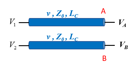
A system of two coupled traces with characteristic impedance Z0, propagation velocity v and a coupling length LC is depicted in Figure 2(a). The voltage at the input to the first trace is an arbitrary voltage V1 and the voltage at the input to the second trace is another arbitrary voltage V2. Since V1 and V2 are any arbitrary voltages, they do not meet the definition of differential signal or common signal components. The goal in the two traces system in Figure 2(a), is to find the voltages at points A and B.
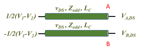
To do that, according to the superposition theory of the DS and the CS, the original problem should be decomposed into 2 sub-problems. In the first sub-problem, the traces are excited with the DSCs ½(V1 – V2) and -½(V1 - V2), and the voltages at points A (VA,DS) and B (VB,DS) are calculated as depicted in Figure 2(b). Since the traces are excited with the DSCs then the impedance of each trace is decreased from Z0 to Zodd and the differential impedance of the traces is Zdiff=2⸱Zodd. The propagation velocity of the DSCs (vDS) will be analyzed in detail later in the article. In the second sub-problem, the traces are excited with the CSCs ½ (V1 + V2), and the voltages at points A (VA,CS) and B (VB,CS) are calculated as depicted in Figure 2(c). Since the traces are excited with the CSCs, then the impedance of each trace increases from Z0 to Zeven, and the common impedance of the traces is Zcom=1/2⸱Zeven. The propagation velocity of the CSCs (vCS) will also be analyzed later in the article.
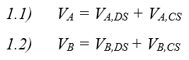
It can be noticed that if the DSC ½(V1 – V2) is summed with the CSC ½(V1 + V2) at the input of the first trace then the original voltage V1 is obtained, and if the DSC -½(V1-V2) is summed with the CSC ½(V1 + V2) at the input of the second trace then the original voltage V2 is obtained. Finally, the voltages at points A and B are a superposition of the two solutions:
 (b)
(b)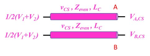 (c)
(c)Figure 2. (a) The original 2 traces problem. (b), (c) The superposition of the DS and the CS. First sub-problem with differential excitation and the second sub-problem with common excitation, respectively.
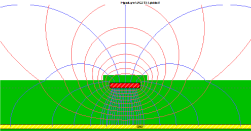
The change in the traces’ impedance due to the DS or the CS excitation is not the main issue in FEXT analysis but rather the propagation velocities vDS and vCS. The Time Delay (TD) of a transmission line (TL) is defined as the time it takes for a signal to propagate from the beginning of the TL to its end. The TD depends on the TL length and on the EM wave propagation velocity. The propagation velocity is the speed that the EM wave propagates in the material. The EM field around a single-ended microstrip is depicted in Figure 3(a).1 In this example, the trace width W=4 mils, the thickness of the dielectric material H=5 mils, the dielectric constant Er=3.8, the thickness of the Solder Mask (SM) that covers the microstrip is tSM =1 mil with dielectric constant ErSM=3.3. Above the SM there is air with dielectric constant Erair =1.
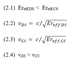
As can be seen in Figure 3(a), the EM field passes through the three dielectric materials and therefore the Effective dielectric constant (Ereff) depends on the three dielectric constants Er, ErSM ,Erair and also on the geometry of the microstrip: H, W and tSM. The value of Ereff will be somewhere between the lowest dielectric constant Erair and the highest dielectric constant Er. Since it is very difficult to calculate Ereff with paper and pencil then a Field Solver is used for that calculation.1 In the example above, the field solver solution for Ereff is 3.025 and hence the propagation velocity v= c / √Ereff =0.57496⸱c, where c is the propagation velocity in a vacuum (3⸱108 m/s or 12 in/ns). Now, another identical microstrip is placed at a distance S of 8 mils from the first microstrip (S is measured between the edges of the traces). The traces are excited once with the DSCs and once with the CSCs. The EM field around the traces is depicted in Figures 3(b) and Figure 3(c), respectively. For these excitations, Ereff is now also depends on the coupling (interaction) between the traces, which is affected mainly by S and H. It can be seen in Figure 3(b) that due to a voltage difference between the traces, the EM field that passes through the air in DS excitation is more significant than in CS excitation (see Figure 3(c)). This fact leads to the conclusion that the effective dielectric constant of the DS (Ereff,DS) is smaller than the effective dielectric constant of the CS (Ereff,CS) (2.1) and therefore the propagation velocity of the DSCs (vDS) (2.2) is higher than the propagation velocity of the CSCs (vCS) (2.3).
For a microstrip:
 (a)
(a)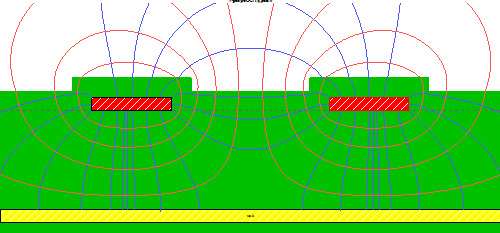 (b)
(b)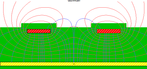 (c)
(c)Figure 3. (a) The EM field around a single-ended microstrip. (b),(c) The EM field around two microstrips excited with DSCs and CSCs, respectively.
The field solver is now used to calculate Ereff,DS and Ereff,CS of two microstrips vs the trace-to-trace separation S at different dielectric thicknesses H (5, 7, and 9 mils). Several calculations and the trends are presented in the graphs in Figure 4.
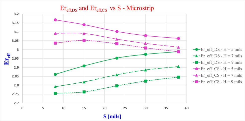 Figure 4. Ereff,DS and Ereff,CS vs. trace-to-trace separation S at different dielectric thicknesses H - two microstrips.
Note: Only the marked points in the graphs were calculated by the field solver. The connection between the marked points is a linear interpolation and does not necessarily present correct values.
At this point the observations from Figure 4 will focus on the impact of S and H on Ereff,DS and Ereff,CS. Later, the impact of S and H on the FEXT will be analyzed.
Observations
- As the separation S between the traces increases, the coupling between the traces decreases. For DS excitation, the EM field in the air between the traces becomes less dominant and therefore Ereff,DS increases. On the other hand, for CS excitation, the EM field begins to get closer to the EM field of a single-ended microstrip, with more EM field lines in the air and therefore Ereff,CS decreases
- When the separation S between the traces is large enough or when H is small enough (high proximity), the traces are loosely coupled so Ereff,DS ≈ Ereff,CS ≈ Ereff
- As H increases (low proximity) more EM field lines will pass through the air and therefore for both, DS and CS, the effective dielectric constant decreases
- In all cases, for a given H, Ereff,DS < Ereff,CS and therefore vDS > vCS.
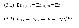
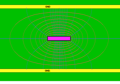
The EM field around a single-ended stripline is depicted in Figure 5(a). It can be seen that the EM field is distributed in the same dielectric material and therefore, the propagation velocity in a single-ended stripline is v=c/√Er. When two striplines are excited with DS or CS (see Figure 5(b) and Figure 5(c), respectively), despite the different distribution of the EM fields, they are still distributed in the same dielectric material and therefore:
for a stripline:
 (a)
(a)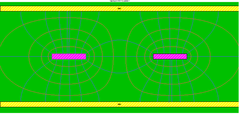 (b)
(b) (c)
(c)Figure 5. (a) The EM field around a single-ended stripline. (b),(c) The EM field around two striplines excited with DS and CS, respectively.
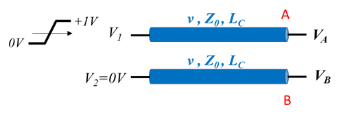
Now, after the superposition theory of the DS and the CS has been presented, and after the propagation velocity of the DSCs and the CSCs in microstrip and stripline have been analyzed, we will turn to analyze the FEXT and its properties. We’ll start with a microstrip. In Figure 6(a), the top trace (trace 1) is the aggressor, the bottom trace (trace 2) is the victim, and their both initial voltage is 0V. The aggressor trace is excited with a step voltage V1 that rises from 0V to +1V during a time of Tr (rise time) while all the other ends of the traces are terminated (V2=0V). The FEXT in this case is the voltage VB at point B and it is actually a response to the step voltage excitation.
According to the superposition theory of the DS and CS, in order to find VB, it is required to decompose this problem into two sub-problems, one with differential excitation, the second with common excitation and the solution to VB is a superposition (sum) of the two solutions (1.2). In the first sub-problem, the traces are excited with the DSCs ½(V1 – V2) and -½(V1 – V2) (see Figure 6(b)) so the propagating signal in trace 1 increases the voltage along the trace from 0V to +0.5V, while the propagating signal in trace 2 decreases the voltage along the trace from 0V to -0.5V. In the second sub-problem, the traces are excited with the CSCs ½(V1 + V2) (see Figure 6(c)) so the propagating signals in traces 1 and 2 increase the voltage along the traces from 0V to +0.5V.
 (a)
(a)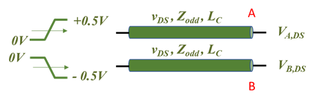 (b)
(b) (c)
(c)Figure 6. (a) The original FEXT problem. (b) The first sub-problem with differential excitation. (c) The second sub-problem with common excitation.
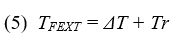
The superposition (summation) of the DSC (green) and the CSC (pink) at point B in a lossless TL are depicted in Figure 7 when the black signal is the FEXT. According to the initial condition of the problem, the initial voltage at point B is 0V. Since for a microstrip vDS > vCS (2.4) then the DSC in trace 2 arrives to point B first after a time of TDDS = LC / vDS and begins to decrease the voltage at point B to a negative voltage. The CSC, which is slower, arrives only after a time of TDCS =LC / vCS. ΔT is defined as the time delay difference between the CSC and the DSC (4). During a time of ΔT the voltage at point B had decreased to a voltage of AFEXT. Starting from time TDCS, the DSC decreases the voltage at point B, while the CSC increases the voltage at the same slew rate - so the total voltage at point B remains constant at AFEXT .This lasts until the DSC finish to fall and reaches -0.5 V (t=TDDS+Tr). From this point, the DSC is fixed at -0.5V, while the CSC voltage still rising, therefore the total voltage at point B start to increase. When the CSC finish to rise and reaches +0.5V (t=ΔT+Tr), and the DSC voltage is already at -0.5V, so the total voltage at point B is a constant 0V. From this point the FEXT will remain 0V.According to the analysis above, the FEXT duration TFEXT (5) can be estimated as:
It also allows to estimate the FEXT amplitude - AFEXT (6) where Vagg and SRagg are the voltage amplitude and the slew-rate of the signal in the aggressor trace:
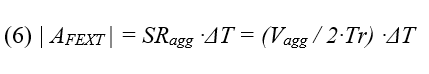
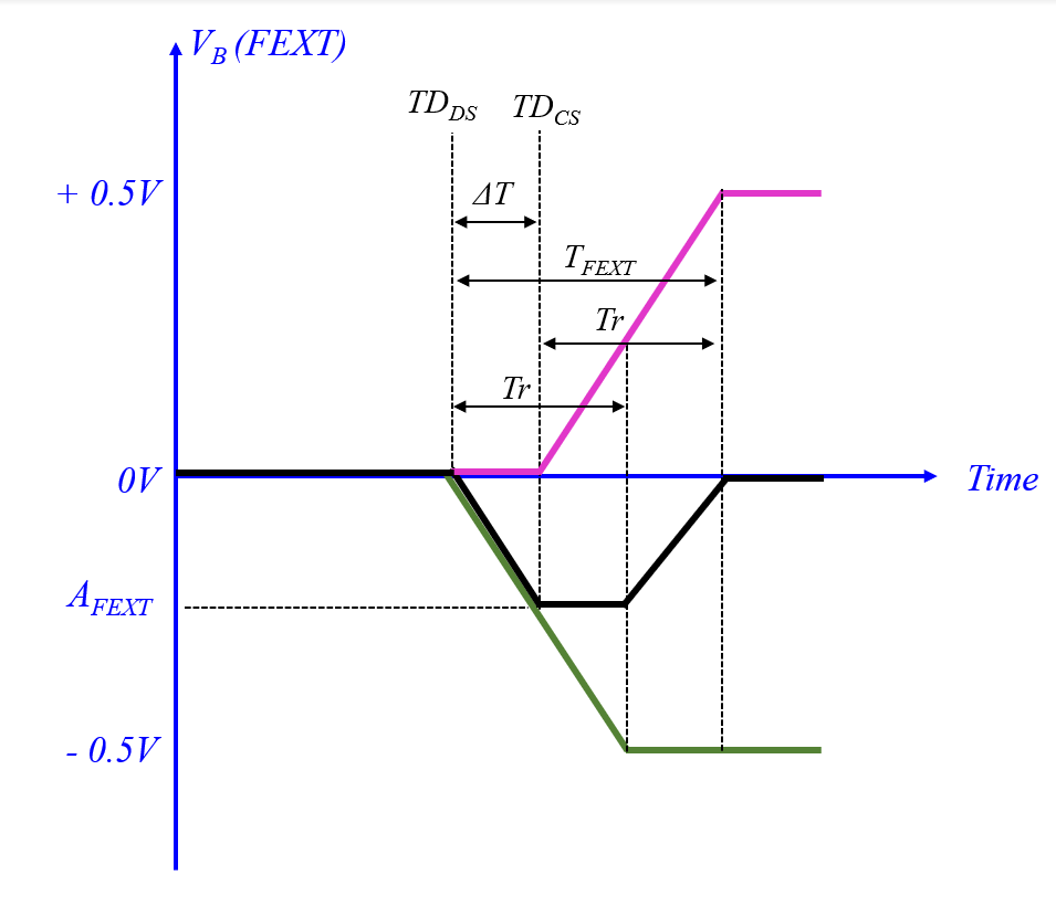 Figure 7. The DSC (green), the CSC (pink) and the FEXT signal (black) at point B.
From the FEXT analysis by superposition of the DS and the CS, several important FEXT properties can be learned:
- The longer the coupling length LC - the higher the FEXT amplitude AFEXT, and vice versa (the snowball effect). This is because as LC increases then ΔT increases as well (4) and during that time the DSC will decrease the FEXT to a lower negative voltage (6).
- The shorter the rise/fall time of signal (higher SRagg) in the aggressor trace - the higher the FEXT amplitude AFEXT, and vice versa. This is because as the slew rate increases then during a time of ΔT the DSC will decrease the FEXT to a lower negative voltage (6).
- In a lossless TL, the maximum FEXT amplitude is half of the signal voltage amplitude Vagg. The FEXT will reach its maximum when ΔT is greater than the signal rise/fall time Tr.
- As the spacing distance S between the aggressor trace and the victim trace increases , the FEXT amplitude decreases, and vice versa. It can be seen in the graphs in Figure 4 that for a given H, as S increases, the difference between Ereff,CS and Ereff,DS decreases. As a result, the difference between vDS and vCS decreases and so does ΔT (4). The smaller ΔT - the smaller AFEXT (6).
- As the dielectric thickness H increases, the FEXT amplitude increases, and vice versa. It can be seen in the graphs in Figure 4 that for a given S, as H increases, the difference between Ereff,CS and Ereff,DS increases as well. As a result, the difference between vDS and vCS increases and so does ΔT. The higher ΔT - the higher AFEXT (6).
- In a stripline, the FEXT amplitude is zero. According to (3.2), for a stripline, vDS = vCS, so ΔT=0 (4). In a stripline, the DSC and the CSC arrive simultaneously to point B. Since they are opposite signals and they have the same slew rate, they cancel each other and the total voltage at point B remains zero, AFEXT = 0. Practically, in a PCB or in a package the average Er around a stripline is a result of the combination of the glass dielectric constant and the resin dielectric constant, so it is not entirely uniform and constant. However, vDS is still approximately equal to vCS, and therefore, in a stripline, the FEXT is significantly lower than in a microstrip.
Note: The calculations above for (5) and (6) are for lossless transmission lines. Loss will cause rise time degradation in both the DSCs and the CSCs and thus will decrease the FEXT amplitude and increase its duration. It also should be remembered that in a casual system like a transmission line, as the loss increases with frequency the dielectric constant decreases in order to keep the system response casual. This fact will cause TDDS in Figure 7 to decrease to a certain extent. Beyond that, all the observations and the conclusions (a) to (f) from the FEXT analysis and Figure 7 are still valid for lossy TL. In addition, it’s worth mentioning that the theory presented above is valid for any two coupled traces. In one case, it could be 2 single-ended coupled traces for FEXT analysis (victim and aggressor), and in another case, it could definitely be a differential pair where one trace is the P line, and the second trace is the N line.
The impact of the rise time on the FEXT properties is demonstrated in Table 1 and in Figure 8 for rise times (0-100%) of 100 pS, 200 pS and 300 pS. In the example, Vagg=1V, lossless microstrip with W=4 mils, H=5 mils, Er=3.8, S=8 mils, LC =6 in (15.24 cm), tSM=1 mil and ErSM=3.3
The DS and the CS propagation velocities were calculated with the field-solver:1
so, for this example:
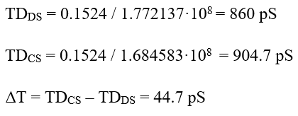
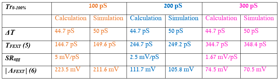 Table 1. The impact of the rise time on the FEXT properties.
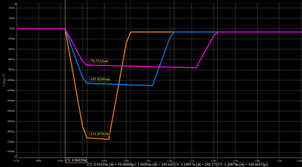 Figure 8. FEXT amplitude and duration vs. the signal rise time: orange – 100 pS, blue – 200 pS, pink – 300 pS.
A good correlation was obtained between the simple expressions for the FEXT duration (5), the FEXT amplitude (6), and the simulation results.
The impact of the coupling length LC on the FEXT properties and the snowball effect are demonstrated in Table 2 and Figure 9. The previous example parameters are taken with 100 pS rise time (SRagg = 5 mV/pS) and Lc = 3, 6 and 9 in.
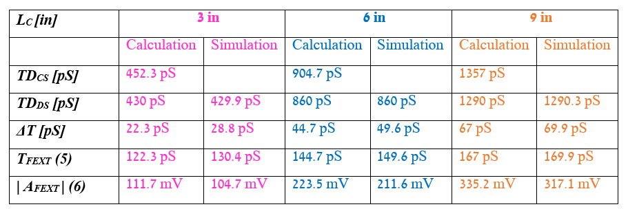 Table 2. The impact of the coupling length LC on the FEXT properties.
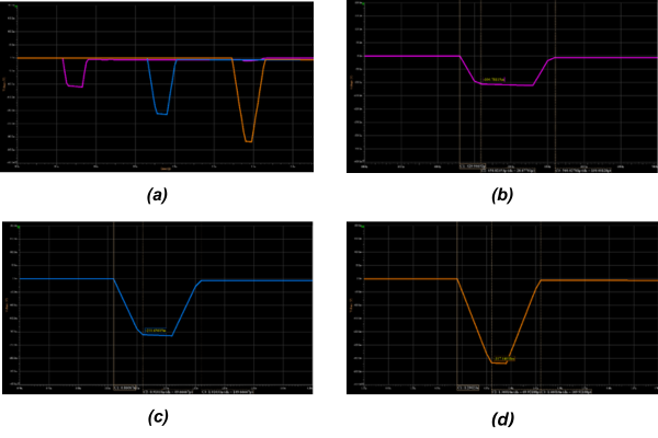 Figure 9. (a) FEXT amplitude and duration vs. the coupling length LC: pink – 3 in., blue – 6 in., orange – 9 in. (b),(c),(d) Zoom in on the FEXT signals for LC=3 in, 6 in. and 9 in., respectively.
 Also, in this example a good correlation was obtained between the simple expressions and the simulation results.
The fact that the FEXT is zero (or practically very low) in stripline is used when routing multiple high data rate lanes. The routing in the internal layers in the stackup is performed in the form of non-interleaved as depicted in Figure 10. If two internal layers are used for the lanes’ routing, then all the Tx differential pairs should be routed in one internal layer and all the Rx differential pairs should be routed in the second internal layer. If only one internal layer is used, then all the Tx differential pairs should be routed in one group (one next to the other) and all the Rx differential pairs should be routed in another group. When routing with stripline, the FEXT is very low and the NEXT is the dominant Xtalk. Hence, it is better that the NEXT will reach the victim’s transmitter and be absorbed by its terminations rather than reaching the victim’s receiver and interfere with the data signal. Of course, even in non-interleaved routing it is still required to maintain a distance of at least 3H between the pairs in order to keep the NEXT low.
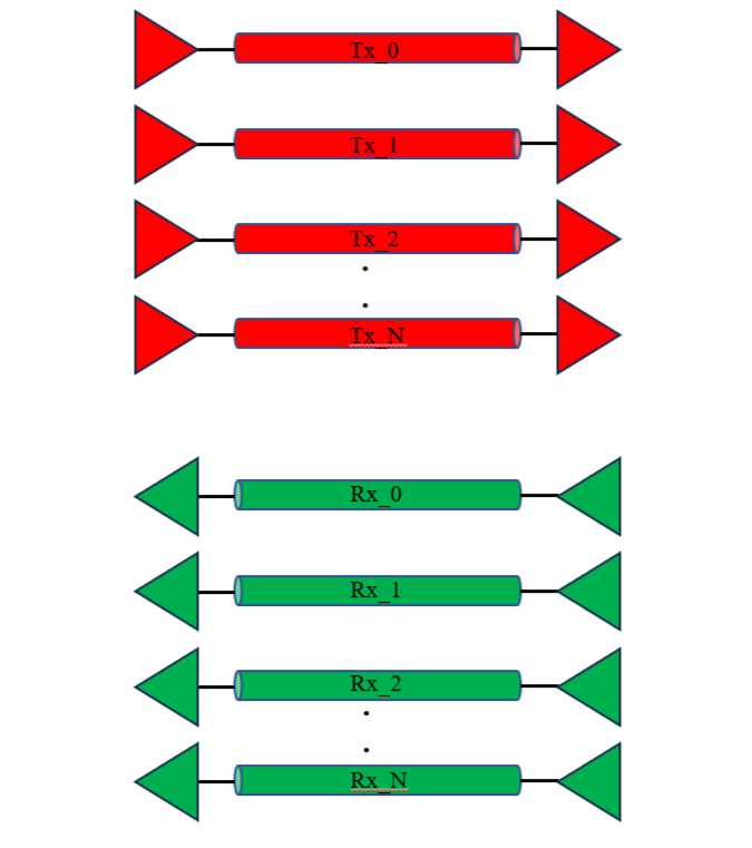 Figure 10. Non-interleaved routing. (Each TL in the picture represents a differential pair.)
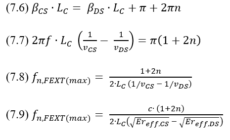
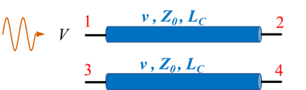
So far, the analysis of FEXT has been presented in the time domain, but the Xtalk components, NEXT and FEXT, can also be analyzed in the frequency domain by using S-parameters. The superposition of the DS and the CS can also be used in this case to estimate at which frequencies the maximum FEXT amplitude is obtained – fn,FEXT(max). In Figure 11(a), port 1 is excited with a sine wave with amplitude V. The voltage coupled to port 4 is the FEXT when ports 2, 3, and 4 are terminated (V2=V3=V4=0). In order to find fn,FEXT(max) at port 4, the problem should be decomposed into two sub-problems. In the first sub-problem, the traces are excited with the DSCs 1/2V and -1/2V as depicted in Figure 11(b). The voltage of the DSC at port 4 in a lossless transmission line is V4,DS (7.1):
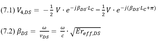
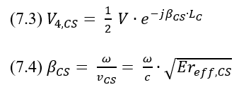
In the second sub-problem, the traces are excited with the CSCs 1/2V as depicted in Figure 11(c). The voltage of the CSC at port 4 in a lossless transmission line is V4,CS (7.3):
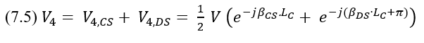
The voltage at port 4 is a superposition of (7.3) and (7.1):
The voltage V4 (FEXT) will reach its maximum amplitude at frequencies where V4,DS and V4, CS will be in-phase:
f0,FEXT(max) (n=0) is the first frequency at which the FEXT amplitude will reach its maximum and it will repeat at frequencies 3⸱f0,FEXT(max), 5⸱f0,FEXT(max),…The frequencies at which the FEXT amplitude will reach its minimum fn,FEXT(min) (7.10) are obtained between the maximum FEXT frequencies such that:

 (a)
(a)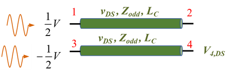 (b)
(b)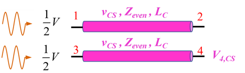 (c)
(c)Figure 11. FEXT analysis in the frequency domain (a) the original problem (b) first sub-problem with differential excitation (c) second sub-problem with common excitation.
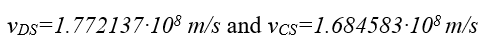
We’ll take the example analyzed in the time domain and calculate fn,FEXT(max) for Lc=0.1524 m. In this problem, the DS and the CS propagation velocities were vDS=1.772137⸱108 m/s and vCS=1.684583⸱108 m/s. According to (7.8), the first (n=0) maximum FEXT magnitude will be obtained at 11.2 GHz and then will repeat at 33.6 GHz, 56 GHz, and so on. In the simulation results in Figure 12, it can be seen that in a lossless transmission line the maximum FEXT (red) is really obtained at frequencies of 11.2 GHz and 33.6 GHz as calculated. At these frequencies, the voltage delivered to port 1 is entirely coupled to port 4 by FEXT and very little is transmitted to port 2 as can be seen in S21 (blue). The pink graph represents the FEXT in a lossy transmission line. The loss caused the maximum FEXT frequencies fn,FEXT(max) to decrease slightly and the FEXT magnitude to decrease substantially. The expressions in (7.8) and (7.9) are still quite accurate, even for a lossy transmission line. Finally, for a stripline vDS = vCS (3.2), so according to (7.8), f0,FEXT(max) will be obtained at an infinite frequency, which means that it practically does not exist, or it is very small.
 Figure 12. S21 (blue) and S41 FEXT (red) in a lossless transmission line. S41 (pink) (FEXT) in a lossy transmission line.
REFERENCES
- HyperLynx SI PI Thermal, VX 2.13 update 1, Siemens Industry Software Inc.