Increasing data rates and reduced margins challenge high-speed link design to step beyond the limits of segmented modeling and co-simulation techniques. The physical transmission layer comprises numerous passive and active components. Their respective interdependencies and trade-offs are not always straightforward to identify.While a channel may pass a test, the remaining margin and thus its resilience against geometry or material variation in production may not be observable. However, such variations are critical because they may impede the performance or cause high volume manufacturing (HVM) products to fail.
For the first time, we developed and demonstrated a polynomial chaos expansion (PCE) flow to analyze a full-featured 100GBASE-KR4 link starting from geometry specification to channel operating margin (COM) margin at the receiver.
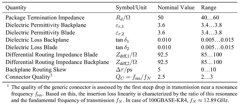
The framework is constructed non-intrusively (see Figure 1). It builds on conventional tools without need for modification and integrates itself into the design flow of established methods. The PCE method is subject to active research and has been successfully applied to investigate aspects of high-speed link design [1, 2, 3]. However, to the knowledge of the authors, the method has not been used in the setting of a practical link design. For instance, the variability of crosstalk between two differential pairs of vias has recently been investigated using PCE and DoE/Response Surface Method (RSM) approaches. A comparison of these two methods is given in [4]. While the the general similarity between the methods is acknowledged therein, the identification of the most influential parameters is not addressed.
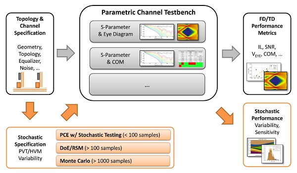
Figure 1: Context and overview of proposed framework for the statistical analysis of high-speed digital links that are subject to process, voltage, temperature (PVT) and high volume manufacturing (HVM) variations. A preprocessing of the specifications expands the analysis and allows for advanced interpretation of results (data flows as indicated by orange arrows). The Polynomial Chaos Expansion (PCE) flow presents itself similar to established methods such as DoE and MCS. Existing solutions for link analysis can be integrated and are summarized under the label Parametric Channel Testbench.
The PCE methodology is, in principal, a variance-based sensitivity analysis, allowing for direct identification of the most influential parameters out of a given set of design or process variations. We statistically analyze the link COM margins and assess its sensitivity and variability with regard to geometry and material variations. Our flow builds on the validated open-source library ChaosPy [5] that implements PCE. Further, we extend ChaosPy by ST [6] to increase the computational efficiency by an a-priori selection of samples. We include relevant Python code snippets and provide guidance for anyone who wants to implement the proposed PCE flow. Moreover, we compare and validate the proposed flow with conventional MCS and DoE based approaches.
Finally, the framework imposes no constraints on the data that is to be analyzed. It allows for a thorough assessment and educational investigation of reference models and compliance metrics such as COM [7, 8]. These are subject to discussion as to which degree they capture the essential causes and effects of link degradation [9, 10]. As increasing data rates continue to reduce the design margins, a comprehensive understanding and prediction of channel performance is crucial. This work addresses this need with a sensitivity-aware assessment of the impact of typical design parameters such as topology, I/O~circuitry, and crosstalk noise.
State of the Art Link Evaluation and Assessment of Parameter Variability
All high-speed links essentially consists of transmitter (Tx), channel (Ch) and a receiver (RX). The ability of a high-speed link to communicate successfully is defined by bit error rate (BER). Validating BER with correct Tx, Ch and RX models is not straightforward, and it is time-consuming. Hence, compliance metrics are introduced as an indirect way to estimate BER without much complexity. Most often, the compliance metrics of Tx, Ch and RX are specified separately such that total link --when concatenated-- achieves the desired BER. Historically, eye height and eye width (or eye mask) at a specified physical location are the absolute metric for compliance validation.
For the interconnect alone, compliance can be specified in terms of frequency domain metrics. In this, key metrics include insertion loss (IL), IL deviation (ILD) and insertion loss to crosstalk ratio (ICR). Most standards specify these compliance metrics as informative guideline values rather than strictly enforced numbers. Recently, IEEE 802.3bj [11, Annex 93A.1] introduced COM as a single compliance metric for the channel validation. It is measured in dB and is defined as

where  represents the equalized signal amplitude, and
  summarizes noise contributors such as transmitter noise (
 TX), residual inter-symbol interference (ISI), timing jitter (J), crosstalk (XT), and receiver equalizer noise (N). It is embraced by other standardization committees such as OIF-CEI, Fibre Channel and JEDEC. The COM computational algorithm is, mathematically, a subset of statistical analysis using single bit pulse responses from S-parameters of the victim and aggressor channels. Compared to full statistical simulators
COM was built on several assumptions that were needed to simplify the algorithm and improve its performance. For instance, the algorithm constraints the fixed feed forward equalizer (FFE) architecture to two or three variable tap coefficients and the continuous time linear equalizer (CTLE) implementation to two or three poles and one or two zeros.
Some areas affected by those simplifications are the computations of input jitter and crosstalk contributions [9]. Moreover, COM considers only two package variations, a short and a long transmission line models. We consider these two cases in the following studies and label them COM short and COM long, respectively.
As data rates increase, high-speed link margins decrease significantly. As a result, validating the channel or link compliance at one design point is inherently risky in high volume manufacturing (HVM) situations. A key metric to assess HVM quality is the number of units fails over a million units produced. This can be equivalently stated as number of links that fail compliance over a million links sampled. Let us define this HVM quality metric as FPM – failures per million. In order to assess FPM, parametric variations of components due to manufacturing tolerances should be included in the link simulation. If the link does not meet a certain FPM target, it is important to rank the most influential variables that impact the compliance metrics and control their manufacturing tolerances. An example of how this quantity can be derived is given later.
Efficient Uncertainty Quantification in High-Speed Link Design
Parametric variations are typically captured through three values: minimum, nominal, and maximum. For a link with N variables, the total number of simulations required would be 3N. Thus, the number of simulations increases exponentially with the number of parameters if we were to simulate all possible combinations. A prudent methodology to reduce the computational burden is to use statistical methods. Monte-Carlo Sampling (MCS) and Design of Experiments (DoE) combined with RSM are two of these methods that are commonly used in industry [12, 13].
MCS is the classical methodology for quantifying variations and their impact on the performance of a digital link. It does not impose any constraints or assumptions on the quantity of interest and uses randomly selected samples out of all possible parameter combinations. However, MCS typically demands a large number of samples to ensure convergence, which can make this technique computationally very expensive. The Response Surface Method (RSM) uses designed experiments to reduce the number of samples and is more efficient in analyzing parameter variability. Based on polynomial regression, a parametric model aims to capture the quantity of interest and its dependencies with regard to the input parameters that are subject to variation. Statistical quantities are derived from the resulting polynomial fit by conventional MCS at lower computational cost.
Note that the distributions of uncertainties in production or design are often known. For instance, Gaussian and uniformly distributed variables cover the common cases of HVM variations and design space exploration. In this paper, we propose a PCE based simulation flow that makes explicit use of this information to boost the efficiency of an analysis. It is inherently well suited for HVM quality assessment and control. Notably, it is computationally more efficient than the conventional MCS and RSM methods in a variety of use cases.
A Survey of Polynomial Chaos Expansion
Similar to RSM, PCE aims to capture the parameter variability by means of a polynomial model from which to derive statistical quantities of interest. Furthermore, both methods make use of specific sampling schemes in order to construct the model. However, one significant difference exists in that PCE is a spectral method. Similar to the Fourier transform that relates time and frequency domain, PCE transforms the deterministic problem at hand into the stochastic domain [14].
In link design, typical quantities of interest include performance metrics such as COM and eye opening. The output quantity varies in accordance with stochastic changes of the input parameters such as geometry and material values. In the following, consider a random variable  that is the output of an arbitrary function
  and depends on an input random variable
  . (In the following text, the function
  and output variable
  are used interchangeably. It should be clear within the given context, which one is meant in either case.) PCE expands this output variable into a truncated series [15, Chap.~5.1]
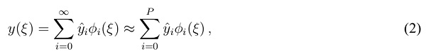
where P is the order of approximation,  denote normalized basis polynomials subject to , and
  refers to the respective PCE coefficient. The sufficiency of a given approximation degree P depends on the smoothness of the function . Generally speaking, the series converges faster for non- or weakly resonant problems which corresponds to a lower P. Increasing P for better accuracy has implications and limitations that are discussed subsequently. The basis polynomials are orthogonal with respect to the inner product [15, Chap. 5.1]

where is the norm,
  is the Kronecker-delta, and
  is the respective probability density function. Given a distribution , the choice of the polynomial basis is set. For the most common cases, these are either Hermite polynomials for Gaussian distributed , or Legendre polynomials in case of uniformly distributed . This finding is fundamental: different random variables of the same distribution only differ in their respective PCE coefficients that characterize the polynomial model. Hence, the PCE coefficients carry all the relevant stochastic information.
When dealing with more than variable, the expression of (2) is adapted to yield [15, Chap.~5.2]
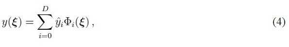
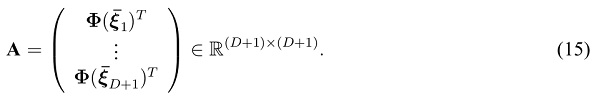
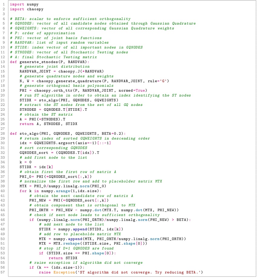
with as the vector of N stochastically independent input random variables. Again,  denote the basis polynomials and the PCE coefficients are given by . Note that the basis polynomials are more general as the previously discussed univariate case. The multivariate, or joint, basis polynomials are obtained from a multiplication of the individual univariate function basis. The number of coefficients in the eventually resulting polynomial model equals (D + 1) and determines the required order D. The required order is given by
  .
.
Various metrics can be derived based on the above PCE formulation. The mean of  equals to the zeroth PCE coefficient, i.e., [15, Chap.~5.3]
and the variance is given by [15, Chap.~5.3]
where the multivariate norms are defined analogous to (3). The values
 are either precomputed or obtained via lookup table. In addition to these well established quantities, conditional variances (Sobol indices) can be derived to analyze the relative impact of the input variability of one or more parameters on the overall output variability. This result comes at no additional cost in PCE, since it can be directly read from the PCE coefficients. The Sobol index corresponding to the
  input random variable
  is [16, 17]
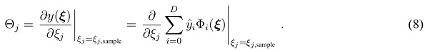
where the index k in the numerator corresponds to relevant contributions with regard to. Note that this primary quantity is unique to PCE. Deriving it from a conventional DoE/RSM model requires significant effort and the accuracy would be limited to that of the RSM model. PCE is free of these constraints thanks to its formulation. Additionally, sensitivities with respect to the input can be obtained through the partial derivative at a sample  analogous to the procedure presented in [18]
Last but not least, the PDF p(y) can be obtained using MCS of the PCE model in the same manner as in DoE/RSM. This is inexpensive since it only involves the evaluation of a polynomial function.
Based on this general outline of PCE, two essential aspects are addressed subsequently: obtaining the PCE coefficients and using as few samples as possible for this. The procedure is illustrated with an example.
Obtaining the Polynomial Chaos Expansion Coefficients
One way to obtain the PCE coefficients is through spectral projection onto the orthogonal basis:
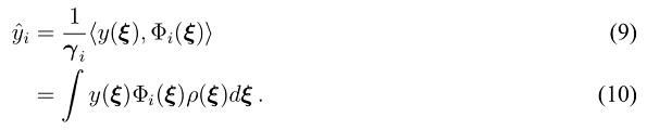
Here, is the joint probability density function. The multidimensional integral for the multivariate case can be solved numerically based on equation (4) using Gaussian quadrature
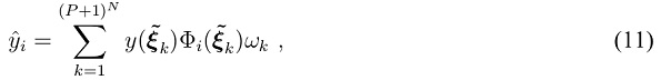
with (P + 1)N being the total number of quadrature nodes obtained via the full tensor product of the quadrature nodes for the univariate case, and  being the corresponding kth quadrature weight. As can be seen from (11), the number of Gaussian quadrature nodes
  and therefore the number of total function calls
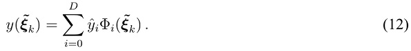
  grows exponentially with N. This is especially detrimental if a single function evaluation, e.g., measurement or simulation, is computationally expensive. Alternatively, point matching equates the function evaluated at a single sampling point
  to the PCE model evaluated at the very same node:
The matching of all sampling points can be written in matrix form
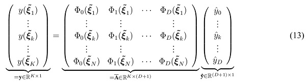
which is an overdetermined problem due to  (D + 1) and linear regression can be used to solve for the coefficients in
  . The next section introduces ST. This method selects the (D + 1) most relevant samples a-priori to further reduce the need for costly function evaluations.
Boosting Computational Efficiency with Stochastic Testing
The ST method [6] uses the aforementioned strategies for obtaining the Polynomial Chaos coefficients. It selects (D + 1) samples that yield maximum possible accuracy for construction of a PCE basis of order P. That is, it selects the stochastically most important nodes.
First, a set of (P + 1)N candidate nodes and their associated weights are set up using the Gaussian quadrature rule as described in (11) through (13). In the next step, the weights are sorted by value. Starting with the greatest weight, the corresponding nodes are successively inserted into the vector of basis functions  ,
,

If any next candidate node yields a new vector that is sufficiently orthogonal to the previously accepted ones, hence, adding to the dimensionality of the matrix  , it is accepted. Otherwise the candidate node is discarded. If from the set of candidate nodes there are D + 1 suitable nodes
  found, we can write once again
This matrix has full rank and is preferably well conditioned. With this, one can write

to obtain the PCE coefficients. Listing 2 explicitly implements this algorithm to demonstrate the extension of the open-source library ChaosPy for use in the proposed framework. The orthogonality of candidate nodes is controlled by a parameter  This value should be a large as possible to ensure a regular matrix . On the other hand, a large value may prevent the algorithm from converging.
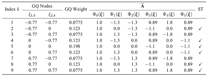
In order to compare the polynomial model obtained from PCE with the result of a conventional DoE/RSM approach, the order of approximation is chosen to be P = 2. This corresponds to a classical choice of a quadratic RSM model. In case of N = 2 independent, uniformly distributed variables  and
and  , Gaussian quadrature yields (2 + 1)2 = 9 nodes as listed in Table 1.
However, the problem is overdetermined. The rank of  equals number of coefficients in the polynomial model. In this example, it is given by
 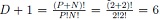 . Hence, three of the nodes need to be eliminated. Within fractions of a second, the ST algorithm selects the rows indicated in Table 1 based on their Gaussian quadrature weight as well as their orthogonality with regard to already selected nodes. Note how
  for all samples. This reveals how the polynomial basis is normalized with regard to
  .
.
Figure 2 illustrates how the two-dimensional domain is sampled and which nodes have been accepted. Figure 3 gives an account of how ST reduces the number of required samples as the number of variables N and the order of approximation P vary.
Computational Cost of Analysis and Normalization of Variables
Two factors may dominate the computational cost of the presented parameter variability analysis: the deterministic analysis of a sample link and the overhead introduced by PCE and ST. This framework acts non-intrusively and does not change or speed up the analysis of a link itself. However, it aims at lowering the total number of required samples in stochastic analysis.
The computation of the stochastic model based on PCE with ST is dominated by the selection of the ST nodes and the projection of deterministic samples  onto the PCE coefficients in (16). Note that the calculation and selection of nodes can be decoupled from the actual samples.
Mapping distributions to normalized intervals, e.g.,  , has two major various benefits without loss of generality: First, the matrix A is independent of the problem. It can be precomputed and tabulated.
Table 1: Gaussian quadrature (GQ) nodes and corresponding weights and rows in . The flag in the last column indicates whether the node is selected by ST.
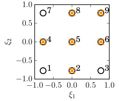
 are depicted as black circles. The index k is printed according to Table 1. Nodes 2, 4, 5, 6, 8, and 9 are selected by the ST algorithm and are highlighted with an orange cross.
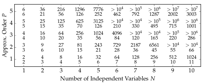
Figure 3: The order of approximation P and the number of stochastically independent variables N govern the required number of samples in PCE. For each tuple (N,P) the grid depicts the evolution of the number of Gaussian quadrature nodes (P + 1)N (upper value) and the number of ST samples 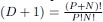 (lower value). It is apparent how ST allows for a large number of independent variables by drastically reducing the number of required samples.
Proposed Modeling Framework
The proposed modeling framework incorporates deterministic analysis methods such as S-parameter extraction, statistical time domain simulation, and COM analysis into a non-intrusive PCE framework as depicted in Figure 4. This allows for integration into any existing work flow.
Two main parts characterize the framework and are discussed in more detail in the following subsections. First, the open-source library ChaosPy, which implements PCE, is extended by the previously introduced sampling technique Stochastic Testing (ST). The second part is an abstract, sensitivity-aware link model. This model serves as an interface between deterministic simulations and PCE. Section 4 demonstrates the framework using a generic 100GBASE-KR4 link without loss of generality.
Implementation of Stochastic Testing
Given the highly modular Python library ChaosPy, it is easy to write wrapper functions in order to condense the use of PCE in combination with ST into essentially four distinct function calls denoted in Listing 1 below.
Listing 1: Obtaining PCE coefficients using the ChaosPy library with ST extention according to Listing 2.

Line 1 obtains the final ST nodes . For this purpose, the function requires two inputs, namely the order of approximation P and a vector of input random variables  . The function is a wrapper function that invokes the core ST algorithm as first formulated in [6]. A corresponding implementation in the Python scripting language is given in Listing 2.
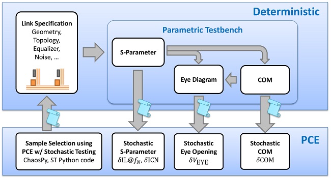
Figure 4: The non-intrusive framework for sensitivity-aware analysis of high-speed digital link comprises a deterministic and a stochastic (PCE) domain. The former can be represented by any conventional analysis of a given link specification. Stochastic quantities are obtained using PCE for pre- and post-processing of samples. The blue scrolls highlight the information exchange between the domains. This study implements the exchange using rudimentary tables of character spaced values. Eye diagrams may be derived directly from extracted S-parameters as well as a COM equivalent [9].
If normalized variables are used, this function call is independent of the actual problem and can be precomputed and tabulated. Obtaining the ST nodes then turns into loading a matrix of rank (D + 1) from a file. The second line represents a wrapper function that invokes the deterministic solver. In essence, this means importing a vector of results, denoted as in (16). Finally, lines 3 and 4 derive the PCE coefficients and a polynomial model. Line 3 corresponds to equation (16). Solving the linear system of equations can be implemented as a LU-decomposition, which can be precomputed, too.
Sensitivity-Aware Link Model
The previously described PCE algorithm is constructed non-intrusively and only requires knowledge of one table of input values and their corresponding output. The table acts as interface between the stochastic and the deterministic domain as illustrated in Figure 4. It maps topological, geometrical, and operational specifications to output quantities such as COM.
In filling the table, conventional measurement, simulation tools and modeling approaches can be selected according to accuracy needs and availability. They do not require any modification. To demonstrate the versatility of the framework, this study uses a mix of tools available to the authors.
The S-parameters of the interconnect are extracted using segmented 2.5D modeling [19, 20]. The COM values and eye diagrams are calculated and validated using a commercial tool as well as publicly available reference implementations.
Listing 2: Python implementation of ST according to [6] for PCE based on the ChaosPy library.
Sensitivity Analysis of a High-Speed Interconnect
Input uncertainty may be due to available design choices as well as unintended parameter variations in production. Both aspects are of interest, albeit at different stages of the fabrication process. Furthermore, it may not always be obvious which parameters are the most influential.
In this section, we demonstrate the capabilities of the proposed framework with a design space exploration. That is, the uncertainties (PDFs) are chosen to feature uniform distributions.
Another popular choice is the normal distribution that corresponds to PVT and HVM uncertainty. The efficiency and accuracy of the framework are validated and put into perspective by comparison with RSM and MCS. For ease of comparison between methods, second order polynomials are obtained from PCE as well as the RSM.
Figures 5a and 5b illustrate the overall link model as well as the considered degrees of freedom. Table 2 summarizes details on the N = 9 independent variables, including nominal values as well as ranges of variation for each parameter, respectively. The total routing length is approximately 21 inch. The stackup and pin assignments are shown in Figure 6.
Note that the dielectric material properties as well as the differential impedance are stochastically independent variables in two of the boards. Blade 1 uses the nominal material properties and routing impedance. The connectors feature the same model.
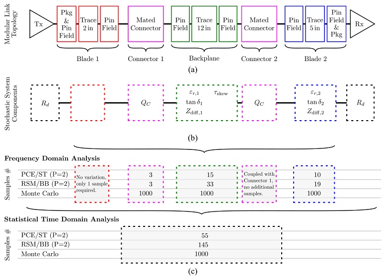
Figure 5: Multiple viewpoints need to be balanced in a variability and sensitivity analysis of a high-speed data link and are depicted in this figure. (a) Topology of a typical backplane link. (b) Values and degrees of freedom considered for the investigation of parameter sensitivity. (c) Number of samples required for different stages of the considered methods and sampling schemes Stochastic Testing (ST) and Box-Behnken (BB). The full number of Monte Carlo samples is required for each partial analysis. This number may vary greatly depending on the required accuracy and quantities of interest.
Table 2: Parameters and their respective ranges as considered in the example design space exploration. The nominal values denote the center value of the respective parameter range.