Fingerprint Your Serial Link to Solve SI

Serial links have focused the practice of signal integrity on managing loss and discontinuities. Each system struggles with one or the other, making it imperative to determine which issue is dominant in your system and respond appropriately. If your interconnect is long, you’ll likely grapple with loss. If it is short and/or modular, minimizing discontinuities becomes imperative. While “long and short” are simplifications that track with “loss and discontinuities” respectively, the challenge of managing their impact on signal integrity requires a deeper look. This article will explain how to characterize, or “fingerprint,” your link to help guide your thinking and solution.

The interplay between loss and discontinuities is interesting, and often non-intuitive. For example, when discontinuities are dominant you can introduce loss to dampen them. Similarly, when loss is dominant, discontinuities have less effect—particularly when they are distant from the Tx and Rx. Noting that Tx/Rx equalization mostly targets loss, discontinuities continue to garner increasing attention. However, in practice, the dance between loss and discontinuities changes with data rate.

Data-Rate Dynamics

Three factors intertwine loss and discontinuities with data rate:

Loss increases with data rate
Size of a relevant discontinuity decreases with data rate
Device equalization capability improves with data rate

Factors one and two explain why SI challenges increase with data rate, while factor three endeavors to mitigate these problems. But be advised that an efficient equalization (EQ) solution for mitigating discontinuities is yet to emerge. In fact, discontinuity mitigation through design is a more identifiable trend than EQ techniques aimed at the same problem. SI best practice begins with eliminating unnecessary discontinuities and then reducing the effects of the ones that remain.¹(See section 2.1.)

Loss concerns tend to dominate 1 to 10 Gb/s signaling due to less available device EQ and the use of higher-loss materials. Discontinuities are dampened by loss and/or remain below the relevant feature size. These data rates cause us to wake up to managing loss, handling it with device EQ or lower-loss materials.

With loss understood and addressed, 10 to 20 Gb/s interfaces are more sensitive to discontinuities. These data rates force us to think about interconnect elements we used to ignore. Via impedance is now relevant, back-drilling non-optional, and connector impedances are carefully characterized—each of these being discontinuities that cause link failures when not managed properly.

For 20-30+ Gb/s, it’s necessary to apply what we have learned at lower data rates and manage both loss and discontinuities. Regardless of PCB material chosen, these frequencies push loss back into the realm of concern.² Furthermore, via and solder pads—and even the stubs resulting from how a device’s pin is soldered down—become discontinuities that must be addressed.

Regardless of data rate and system type, managing the interplay of loss and discontinuities is necessary to preserve signal integrity. As such, it’s important to fingerprint your link to determine if it leans towards lossy or reflective.

Determining Your System Type

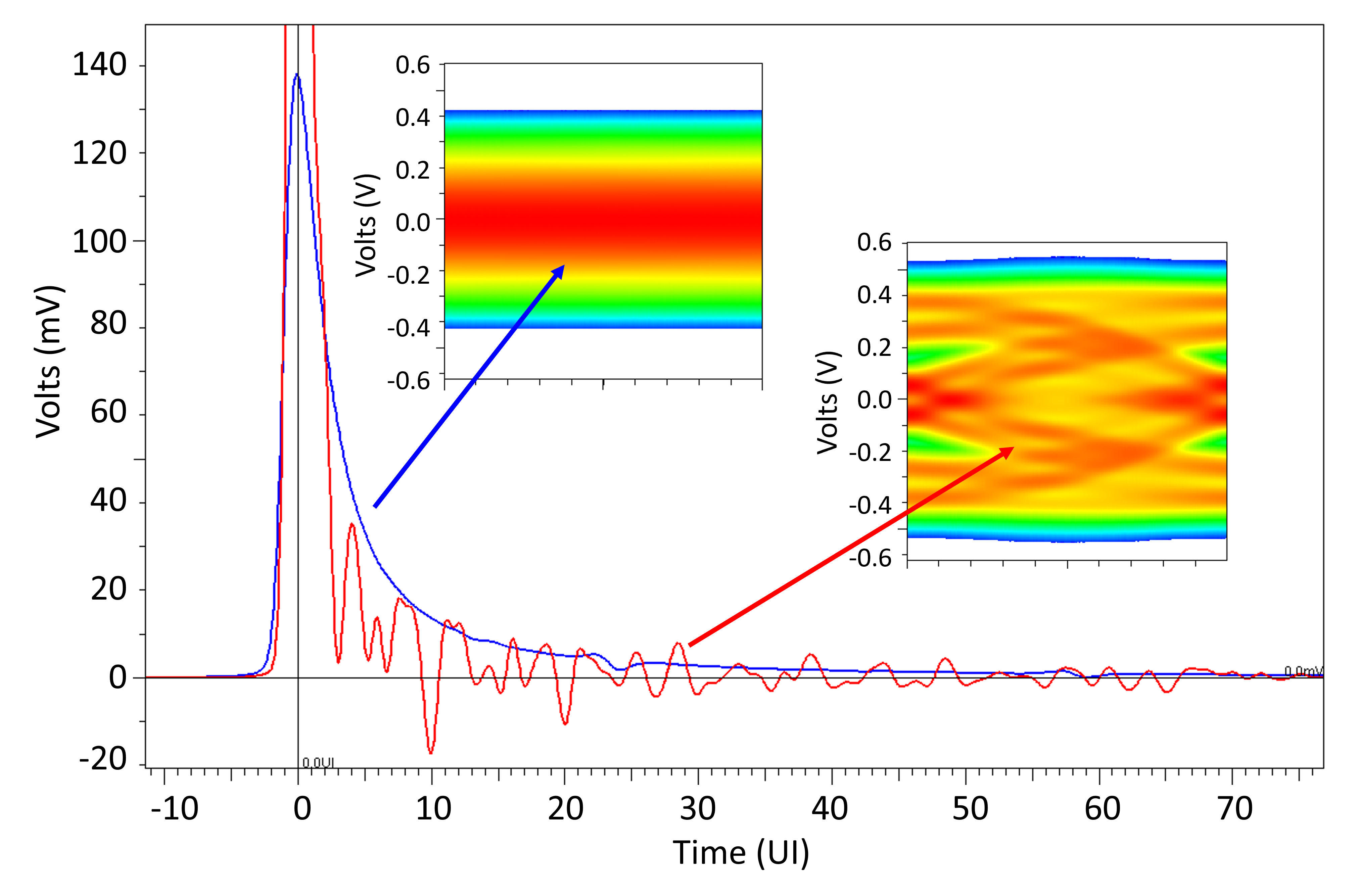
Your SI effort becomes better focused when you determine which type of system you have: lossy or reflective (i.e., discontinuity-dominant). To illustrate the two types of systems, Figure 1 and Figure 2 highlight their characteristic differences. Even though the lossy system (blue) is four times longer than the reflective system (red), both produce closed eyes—further demonstrating that both issues must be understood and addressed.

An interconnect’s pulse response (see Figure 1) is its fingerprint that reveals its identity, and hence its leaning towards lossy or reflective. Lossy interconnects have a lower-amplitude pulse at UI 0.0, followed by a slow and continuous decay that requires multiple UI to return to 0 V. Conversely, discontinuities allow substantial pulse amplitude (400+ mV, in this case,) followed by reflections that cause ringing around the 0 volt line for multiple UI. Both channels accumulate significant interference and pulse spreading into unintended bit times, with each one showing millivolt level interference beyond 60 UI (X axis tick marks). Quantitatively, eye height is mathematically reduced by subtracting the pulse response’s difference from 0 V at each UI outside the primary bit (UI 0.0). While a typical channel’s pulse response may be a blend of these characteristics, these examples clarify how both problems appear within the interconnect’s fingerprint.

Figure 1. Loss (blue) and discontinuity (red) channel fingerprints. (All figures/plots created in MATLAB and Signal Integrity Toolbox.)

Loss plots (see Figure 2) provide additional insight into channel characteristics. Differential Insertion Loss (IL), illustrated in darker shades, reveals the lossy channel, illustrated in blue, has three times more loss than the reflective channel. While IL non-linearity (sometimes called “Insertion Loss Deviation”) suggests the red channel is more reflective, its differential Return Loss (RL) makes that point quite clear. RL is a direct measure of reflected energy, showing the reflective channel, illustrated in light red, exceeds 10 dB around 3 GHz. (10 dB is a common RL metric identifying the frequency where reflections can become problematic.) In contrast, the lossy channel’s RL, illustrated in light blue, stays below 16 dB at all frequencies.

While active metrics (e.g., eye opening, BER) are the ultimate judge of channel performance, the items in Figure 1 and Figure 2 and other passive metrics can inform and guide your channel design. For example, TDR plots reveal each discontinuity’s magnitude and location.³ System design is optimized by using tools to explore, iterate, and manage the effects of loss and discontinuities through studying these types of plots.

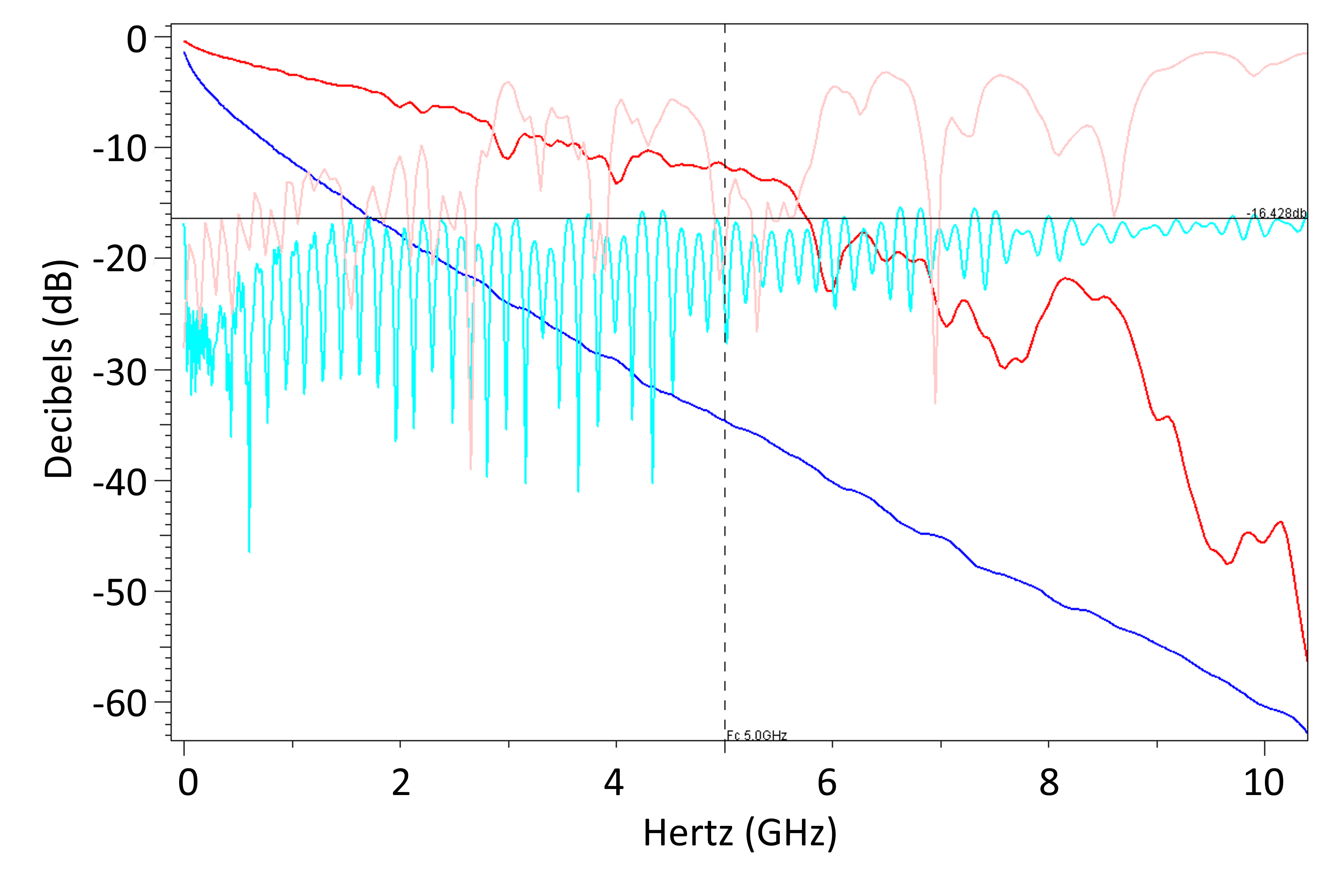Figure 2. IL/RL in lossy (blue) and discontinuity (red) channels.

Given the ability to identify and differentiate loss and discontinuities, let’s have a closer look at how they are interrelated.

Trading Loss and Discontinuities

Trends of increasing integration and product miniaturization continue to shorten interconnects, making the majority of channels more reflective than lossy. As such, modern link failures tend to be caused by discontinuities.¹ (See pp. 95.) How can discontinuities be corrected? Discontinuities are removed by matching the impedances of the items in your channel (such as traces, vias, connectors, and packages) to each other. But sometimes—particularly with connectors—a discontinuity cannot be removed. As such, it becomes a feature you must manage.

One solution for managing discontinuities is not intuitive: add loss to your system. After decades of trying to minimize loss, in many cases we have over-achieved and inadvertently maximized the impact of discontinuities. As such, using low-loss materials and shortening traces is not always the best choice. Adding loss reduces reflections due to discontinuities, just as damping reduces ringing.

As an example of using loss to dampen reflections, Figure 3 shows Gen4 PCIe® eye height and width margins versus system implementation options, which are illustrated in different colors. Zero margin is the black horizontal line in each plot, and positive margin increases vertically upward. This is a short 3-PCB system with typical connector discontinuities between them. The design scenario allows us to influence two of the PCBs while one is fixed. Route lengths on two PCBs are tested at both 1 in. (red/green) and 3 in. (blue/gold), revealing that longer length doubles height and width margins. What? Let me say that again. Tripling the length doubled the margin. This is not intuitive, yet occurs in numerous situations when discontinuities dominate loss.⁴ Obviously, at some point, increasing length will no longer increase margin, but in this length range, the longer routes offer substantial improvement.

Figure 3. PCIe Gen4 eye height (left) and width (right) margins vs. Tx preset and L=length/Df options.Figure 3 additionally compares the effects of dielectric loss. Adding loss to the 1 in. lengths (Df: red = 0.005, green = 0.02) not only improves margin, but also linearizes performance across Tx EQ Preset options (X axis). Though PCIe does not require margin to multiple presets, linearity suggests a more stable system and immunity to EQ training inefficiency. Figure 3’s margins for the 3 in. lengths (blue/gold) illustrate another phenomenon related to trading loss and discontinuities. Note that the higher loss material (Df: gold = 0.02, blue = 0.005) shows better margin in width, but not in height. In general, loss limits eye height (amplitude) while its damping improves eye width (jitter). In a reflective channel, discontinuities exacerbate deterministic jitter, hence eye width is observed to improve as an intermediate amount of damping loss is introduced.⁵

While eye height and width are interrelated, the common dynamic shown in Figure 3 provides an opportunity to place the margin where it is needed most. In this scenario, the margin reversal is not true at the 1 in. length, yet at the 3 in. length damping from the higher-loss material starts reducing eye height while still improving the reflective jitter for better eye width. Choosing the best trade-off between length and Df requires testing the range of options and engineering judgment.

Discontinuity or Impedance?

Another non-intuitive design option is choosing to match a serial link’s natural impedance instead of its specified impedance. In other words, it can be more important to minimize discontinuities than achieve a standard impedance at various points throughout the channel. For example, if a 100 Ω connector must be used in an 85 Ω system, consider implementing the whole system at 100 Ω . And vice versa. When a signal path traverses required discontinuities and then returns to a supposed “correct” impedance, more discontinuities are created. Allow yourself the freedom to simply minimize discontinuities, using a good simulator to explore and validate your choices.

In Conclusion

Advancing serial links through generations of data rates increasingly requires managing—if not trading—loss and discontinuities. Common metrics such as IL, RL, and pulse response help fingerprint the interconnect to understand how, and to what extent, the two problems are limiting a channel’s performance. While device equalization typically handles loss, discontinuity-induced link failures can be corrected using non-intuitive solutions such as adding length or loss and adapting standard impedance values. Try fingerprinting your channel using this free trial of MATLAB’s Signal Integrity Toolbox.

This article is an excerpt from Donald Telian’s book, Signal Integrity, In Practice: A Practical Handbook for Hardware, SI, FPGA, and Layout Engineers.

REFERENCES

- D. Telian, Signal Integrity, In Practice: A Practical Handbook for Hardware, SI, FPGA & Layout Engineers, 2021.
- D. Telian, K. Rowett, I. Teplitsky, "PCIe Gen5 Signal Integrity Implementation – Issues & Solutions," DesignCon, 2023, Figure 1.
- M. Steinberger, "Understanding TDR," 2012.
- D. Telian, S. Camerlo, B. Kirk, "Simulation Techniques for 6+ Gbps Serial Links," DesignCon, 2010, pp. 20.
- D. Telian, "Discontinuity Proximity Effect," Signal Integrity Journal, November 7, 2023.