
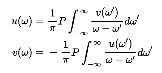
Most of us bringing Touchstone channel models into our time domain link simulations have been advised to enforce the Kramers-Kronig relations before converting to the time domain:
(1)
where:
- u(ω) is the real part of the frequency response,
- v(ω) is the imaginary part of the frequency response, and
- P is the Cauchy principal value operator, used to evaluate improper integrals, such as those above.
We are told doing so will ensure our channel impulse response remains causal, a critical necessity for accurate link modeling. Additionally, we often wonder, “where did those come from?”
Well, they are not hard to understand if we start where the actual story starts: the time domain, and a very clever way to absolutely guarantee a signal is causal (i.e. - zero for time, t < 0). Since we tend to do better engineering when we understand the reasoning behind things, it is worth going through this exercise to see where these relationships come from.
Something we must remain cognizant of as we proceed: (1) presumes that we know our response at all frequencies. Of course, this is seldom the case when we are limited by simulator and/or measurement finite bandwidth. Keep in mind:
- As long as our simulation/measurement extends to a frequency at which the magnitude of the response has dropped sufficiently, the error introduced into (1) by non-infinite integration should be slight.
- Regardless of the error introduced by non-infinite integration, it is still valuable to our engineering intuition to connect the Kramers-Kronig relationship expressed in the frequency domain to its time domain equivalent, as that was the actual starting point for this article.
Time Domain Specification
Let us assume the signal is decomposed to even and odd components:
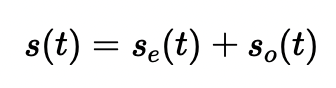
(2)
where:
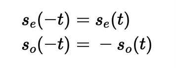
(3)
Then we can enforce causality, as follows:
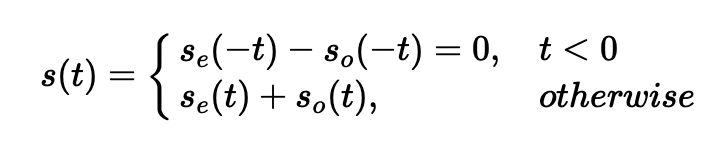
(4)
which we can satisfy by requiring:
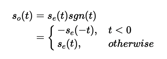
(5)
Note that this also implies: 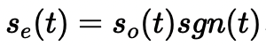 (6)
(6)
And we have:
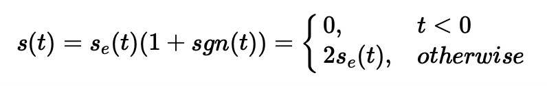
(7)
which is causal by definition.
Frequency Domain Consequences
What are the resultant consequences to the spectrum of such a signal?
Well, we know that:
(8)
where 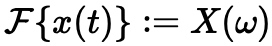 (9) is the Fourier transform of x(t), defined as:
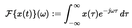
(10)
And we know that multiplication in the time domain is equivalent to convolution in the frequency domain.
So, we have:
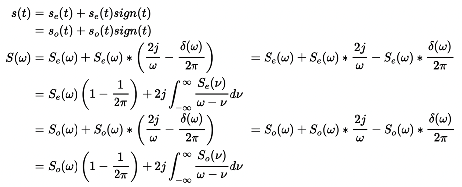
(11)
And we finish by observing that:
The Fourier transform of an even function is purely real:
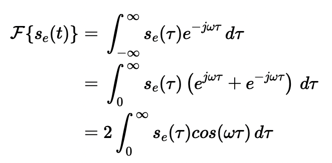
(12)
The Fourier transform of an odd function is purely imaginary:
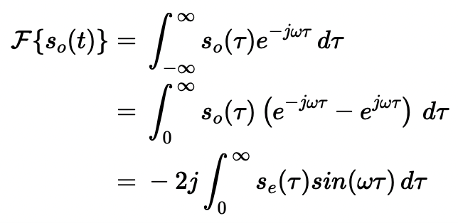
(13)
This tells us that:
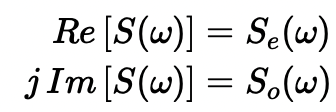
(14)
And using this to rewrite the definition of S(w):
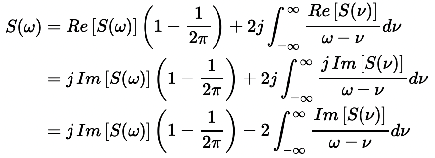
(15)
Equating the real and imaginary parts of the two expressions for S(w) gives us the Kramers-Kronig relation:
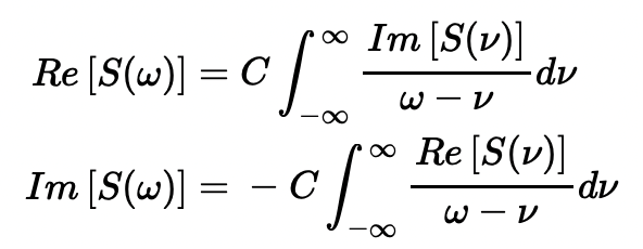
(16)
where:
(17)
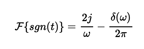
The multiplicative constant differs from the usually stated form of the Kramers-Kronig relation, because we have used the more correct form of  , which includes the subtractive delta function, normally omitted by most authors.
(It is not hard to convince yourself this form is more correct, by simply observing that the "d.c." component of the spectrum of the sgn(t) function must be zero.)
Conclusion
By starting where the actual story began in the time domain, we have made the Kramers-Kronig relations less of a mystery and provided a more intuitive grasp of the motivation for their derivation.