
Few topics are as fundamental in signal integrity and create as much confusion as signal bandwidth. What exactly does bandwidth refer to and what features in the time domain influence bandwidth; rise time or slew rate?
For the two waveforms in Figure 1, what are their bandwidths and which waveform has the higher bandwidth? The answer may surprise you. This is an important question because it applies to all analysis in the frequency and time domains for both simulation and measurement.
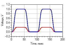
Fig. 1 Two waveforms have the same rise time but a factor of 5 different slew rate. Which one has the higher bandwidth?
While the term bandwidth is used when referring to the frequency components of a signal, it has an ambiguous definition that must be clarified before it can be applied to help gain insight into its relationship with rise time and slew rate. Bandwidth is, fundamentally, the frequency range of a signal’s “significant” spectral components.
When applied to RF signals, this is generally the range of frequency components in the spectrum about the carrier frequency and is often categorized as narrow band or wide band. For digital signals, since their frequency range starts at DC, bandwidth refers to the highest sinusoidal frequency component of the signal that is “significant.” The ambiguity is in the definition of “significant.” Just looking at the spectral components of a time domain signal in the frequency domain is not enough to answer the question “what is significant?”
Time Domain Waveform Representation in the Frequency Domain
A time domain signal is generally transformed into the frequency domain with a Fast Fourier Transform (FFT), which is a fast matrix solution of a Discrete Fourier Transform (DFT). This changes a time domain V(t) waveform into a frequency domain spectrum consisting of a complex sinusoidal amplitude in each spectral frequency bin, A(f). Only the magnitude of the complex amplitude is generally displayed, but there is an associated phase as well.
There are three features in the time domain waveform that translate directly into features in the frequency domain. These apply to an FFT of a waveform whether the waveform is simulated or measured.
- The spectrum is calculated by sampling the waveform over a finite span with an acquisition window. The acquisition window is a time interval which repeats. The first frequency component above DC and the interval between frequency bins, frequency resolution, are related to the total acquisition time over which V(t) data is simulated or recorded. If the total time window is 1 usec, the frequency interval between each bin (i.e. frequency resolution) is 1/1 usec = 1 MHz.
- The average value of V(t) in the time domain, over the acquisition window, is the amplitude of the DC component, the 0 Hz frequency bin, in the frequency domain spectrum. For example, if the average in the time domain is 0.5 V, the amplitude of the 0 Hz frequency component is also 0.5 V.
- The highest frequency bin in the spectrum is ½ the sample rate of the measured or simulated data in the time domain. If the sample rate is 100 GHz, the highest frequency component that can be calculated with an FFT is 50 GHz.
The FFT of an ideal sine wave in the time domain yields just one sinusoidal frequency component, the sine wave’s frequency. For example, the spectrum of three ideal sine waves at 10 MHz, 100 MHz, and 1 GHz calculated with the FFT function in Keysight’s Advanced Design System (ADS) is shown in Figure 2. The time base is 1 usec and the sample interval is 5 psec for a resolution of 1 MHz. The highest displayed frequency is 100 GHz. For this example, a Blackman-Harris window is used in the FFT.
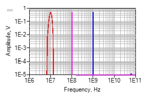
Fig. 2 Simulated FFT of three ideal sine waves each with an amplitude of 0.5. Note the resolution is 1 MHz.
It is obvious from this example that the highest significant spectral component of a sine wave is just the sine wave frequency itself. The amplitudes of the frequency components shown above the sine wave frequency are at the numerical noise floor of the FFT and are insignificant.
The Ideal Square Wave
One of the few waveforms that allows pencil and paper calculation of an FFT is an ideal square wave. The spectral components are multiples of the repeat frequency, the fundamental. Each multiple of the fundamental is a harmonic. Their amplitudes drop off as 1/n and are related by: 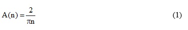 Where:
A(n) is the amplitude of each frequency component and n is the harmonic number, a multiple of the first harmonic frequency.
In the special case of a perfectly symmetric square wave, all the even number harmonics in the spectrum cancel out and are numerically equal to 0. Any asymmetry between the first half and the second half of the waveform creates some even harmonic components. A second harmonic component in the spectrum of a periodic square wave-like waveform means that the measured square wave has some asymmetry between the first and second half of its period.
A simple check of any FFT tool is how well an ideal square wave’s calculated spectrum matches the ideal analytical calculation (see Figure 3). In this example, the square wave has a 5 psec rise time (the sample interval) and has a perfectly symmetrical 50 percent duty cycle. This is compared with the same square wave but with a 50.1 percent duty cycle.

Fig. 3 An ideal square wave's spectrum compared with the analytical model and the impact of a slight asymmetry in the waveform.
From the spectrum of the ideal square wave, how is bandwidth defined? The frequency components drop off in amplitude by 1/f and become arbitrarily small. Below what amplitude are the frequency components insignificant? One must be careful applying a definition such as the 3 dB bandwidth (the frequency at which the amplitude is down by 3 dB). This is simply an amplitude drop to 70 percent of the starting value. The first harmonic is already down to 63 percent of the peak-to-peak value of the square wave’s voltage. The third harmonic is down to 33 percent or almost – 10 dB from the first harmonic. This is for an ideal square wave with a 5 psec rise time in this example.
The amplitudes of the harmonics in the signal’s spectrum are not what is important. It is the highest frequency required to describe the rise time of the signal. In this ideal square wave, with a 5 psec rise time, all the frequency components displayed are important, however tiny in amplitude. Not including some range of frequency components means not replicating the 5 psec rise time. The amplitude of a frequency component in the spectrum of a signal, or the relative amplitude changes of the spectral components is not enough to define the bandwidth.
Synthesizing a Finite Rise Time Square Wave
Another way of evaluating the bandwidth of a signal, the highest significant sinusoidal frequency component, is to synthesize a square wave with a finite rise time and an unambiguous bandwidth. A square wave can be created by successively adding together each frequency component from its ideal spectrum, starting with the lowest harmonic, one at a time.
The spectrum identifies the frequency components and their amplitudes. A pattern of frequency components containing other than the amplitude A(n) = 2/(pn) will not yield a square wave. It will be some distorted repetitive signal. The amplitudes must drop off as 1/n to create a signal resembling a square wave.
Multiple sine waves of different frequencies can be simulated in the time domain and added together using a simple circuit with ideal sine wave voltage sources in series. Using the analytically calculated amplitudes of an ideal 100 MHz square wave, Figure 4 shows the circuit and the resulting time domain waveforms for the first 17 harmonic components added together. The fundamental is 100 MHz and each harmonic is a multiple of 100 MHz. The amplitudes of the even harmonics are 0. As higher frequency components are added to the waveform, the rise time of the resulting signal decreases; they are inversely related.

Fig. 4 Example of part of the circuit used to add together sine wave frequency components in Keysight's ADS and the resulting synthesized waveforms.
The bandwidth of each composite waveform is unambiguous. The highest sinusoidal frequency component that is significant in each waveform is the highest sine wave that is added. Even though the amplitudes of each higher frequency component are smaller and smaller, each additional component is critically important in enabling a shorter rise time.
For example, the waveform with the first 17 harmonic components and the resulting spectrum of this time domain waveform are shown in Figure 5. The bandwidth of this waveform is engineered to be 1.7 GHz.

(a) (b)
Fig. 5 The center portion of the waveform containing the first 17 harmonics of an ideal 100 MHz square wave (a) and the engineered spectrum (b). Note the bandwidth is exactly 1.7 GHz, with no ambiguity. This is the highest sinusoidal frequency component in the waveform.
This ADS simulation can be used to perform a simple numerical experiment in which the 10 to 90 percent rise time of each engineered waveform is compared to its engineered bandwidth. The relationship between the 10 to 90 percent rise time and the engineered bandwidth is shown in Figure 6 compared to the commonly used approximation, RT = 0.35/BW. Rise time and bandwidth are inversely related. A useful figure of merit for this relationship is the rise time-bandwidth product. In this numerical experiment, each term is unambiguously defined. This product, as the harmonic number is increased, is also shown in Figure 6.

(a) (b)
Fig. 6 Measured rise time (circles) and the common approximation (line) (a). Actual rise time-bandwidth product for the synthesized finite rise time square wave (b).
The data points plotted in Figure 6 show a purely empirical relationship based on a numerical experiment that unambiguously defines the highest frequency required to replicate a specific rise time. The value of the rise time-bandwidth product depends strongly on the precise shape of the rising edge.
The commonly used model relating rise time and bandwidth is a good approximation for the results of this numerical experiment, however, it is only an approximation. This model is derived based on the ideal step response of a 1-pole filter. In this model, the 1-pole frequency is “arbitrarily” defined as the bandwidth of the signal. In comparison with the unambiguous definition of bandwidth based on the empirical experiment, this assumption is reasonable. The rise time-bandwidth product in the empirical experiment ranges from 0.2 to about 0.42. The value of 0.35 for the 1-pole model is an approximation that fits within this range.
Rise Time and a 1-pole Filter Response
The empirical relationship between rise time and bandwidth based on the engineered spectrum matches the simple 1-pole filter response model if the bandwidth of the signal is defined as the pole frequency. This suggests there is something special about using the pole frequency of a 1-pole filter as the bandwidth of the signal.
A 1-pole low pass filter has a transfer function of 0 dB at low frequency. At the pole frequency, the transfer function drops to – 3 dB; and thereafter, the transfer function drops by 20 dB/decade. This means that when an ideal square wave spectrum passes through a 1-pole filter, the amplitude of the frequency components at the pole frequency are down by 3 dB (an amplitude drop to 70 percent of the original value) with a drop off much faster above the pole frequency. The pole frequency is a good figure of merit for the frequency at which the harmonic amplitudes begin to drop off and quickly become insignificant.