Every RF engineer learns about the Smith Chart their first day studying S-parameters. It’s an important tool for RF applications. Not so for SI applications. But there are some valuable insights a Smith Chart can illuminate.  Here’s how to extract those few nuggets.

Let’s Start with Reflections

Each S-parameter is really the ratio of the sine wave voltage signal coming out of the end of an interconnect, relative to the sine wave voltage signal going in. We call the ends ports. For now, we will consider only one port connected to the interconnect, or device under test (DUT).  The DUT can be anything, even a discrete component like a resistor or capacitor, or an extended structure like a transmission line, traces on a board or an entire channel. Figure 1 illustrates this idea of an incident and reflected sine wave signal from a DUT.

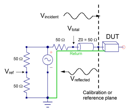
Figure 1. Establishing the incident signal, which is the same as Vref, and the reflected signal from a DUT.

S-parameters can come from measurements or simulations. Regardless, their properties and the information we extract from them, are the same. We label each specific S-parameter term based on the port number of the going in port and the coming out port. When there is only one port, the only S-parameter term is S11. It is the ratio of the reflected wave to the incident wave. We call this the reflection coefficient and also, for historical reasons, the return loss.

The ONLY way a signal going into port 1 can come back out port 1 is due to a reflection, somewhere in the DUT. The ONLY thing that can cause a reflection is an impedance change. This means there is valuable information about the impedance structure of a DUT buried in S11.

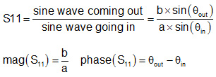
Since we are describing sine waves of signals entering and leaving a DUT, we have to keep track of the frequency, the amplitude and the phase of each wave. When we take the ratio of the sine wave reflected to the sine wave incident, we end up with two numbers, the ratio of the amplitudes of the two waves and the difference between the reflected wave’s phase minus the incident wave’s phase:

Let’s take as an initial example, the return loss from a uniform, lossless, 50 Ohm transmission line, open at the far end. What do we expect S11 to look like?

Since the line is lossless, whatever we send in, should come back out, so the magnitude of S11 should always be 1. It’s the phase that will change. We send a signal into the front of the line. The signal travels to the end of the line, sees the open, reflects, with no phase shift, and makes its way back out of the line into the port.

The phase coming out now is not the same was the phase going in, now. The phase going in, now, has advanced ahead in the time it took the sine wave to travel through the transmission line. This means the phase of S11 will be negative and it get larger, and more negative as we increase frequency.

At the lowest frequency, the phase difference going in and coming out will be very small. On a polar plot, S11 should start on the far-right edge of the circle, where the magnitude is 1 and the angle with the real axis is close to 0 degrees.

As we increase frequency, the phase increases in a negative direction and S11 moves along the unit circle in the clockwise direction.

If there is a little loss in the line, which increases as we increase frequency, the S11 will appear to spiral into the center as it rotates around in the clockwise direction. This is what the return loss would look like on a polar plot.

We can also describe the two numbers that are part of S11 at each frequency, as a real and imaginary term, a magnitude, in dB, and phase in degrees at each frequency, or plotted on a polar plot. As an example, these three types of plots, for the same lossy transmission line, are shown in Figure 2.

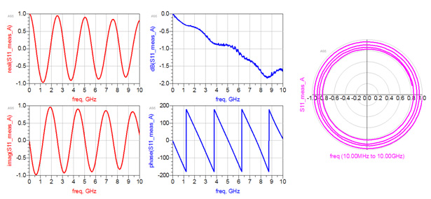
Figure 2. Examples of the three ways of plotting S11. Left: real and imaginary, middle: magnitude in dB and phase in degrees, Right: polar plot.

This is an example of the measured data from a short transmission line structure. The data is exactly the same in each case, yet, it looks very different depending on how it is plotted. The only reason we plot data is to look for patterns and immediately interpret the results. Which plot we use depends on what question we are asking and which one gets us to the answer faster.

Notice that in the two plots with the frequency axis, we can get a good measure of the precise value of each term at any frequency. But when plotting the return loss on a polar plot, we lost the specific frequency information. We would have to place a marker on the graph to tell us where each frequency value is located in the spiral curve. However, there is value looking at the pattern of S11 in the polar plot.

Analyzing Reflections

The only thing that causes a reflection is a change in impedance. As the incident sine wave signal transitions from the port to the DUT, it will see an input impedance related to the entire DUT structure. The impedance mismatch between the 50 Ohms of the port and the net, total, integrated impedance of the DUT. The value of S11 can literally be calculated from

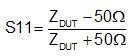
In this case, the input impedance of the DUT is complex and S11 will be complex. One of the nuggets of value in looking at S11 in the polar plot. In this plot, the location of any displayed point is has a magnitude as the length of the vector to that point, and the angle the vector makes with the real axis as the angle.

The value of the polar plot is from patterns the return loss makes for different DUT structures.

Patterns in the Return Loss

Let’s consider the patterns created on a polar plot for the return loss from a variety of different structures. Some aspects of the pattern S11 will make on a polar plot can be predicted using the analytical equation above.

First consider an ideal open. The reflection coefficient from an open is always +1. It is real with no imaginary component. Plotted on a polar plot it is a point, at all frequencies on the far-right side of the polar circle.

A short, likewise, is always -1 and is plotted on the real axis as well, on the far-left side of the circle.

For an ideal resistor element with a resistance of R. What will the return loss look like at any frequency? Since the resistance is constant with frequency, the return loss will have the same value at every frequency. The analytical solution is just

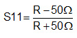
The result is just a number. It is only real, as there is no imaginary component. This means, when plotted on the polar plot, S11 will only be on the real axis. When R is greater than 50 Ohms, S11 is a number from 0 to 1. When R is less than 50 Ohms, S11 is a negative number from 0 to -1.  And, S11 is constant with frequency. There will only be one value for all frequencies. Figure 3 shows the return loss of an open, short and three resistor values on a polar plot across a large frequency range. Note the patterns.

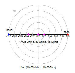
Figure 3. the S11 of an open, short and three different value resistors on a polar plot.

If you ever see S11 on a polar plot, touching the real axis, you know it has an impedance that looks like an ideal resistor.

The S11 from an ideal capacitor is

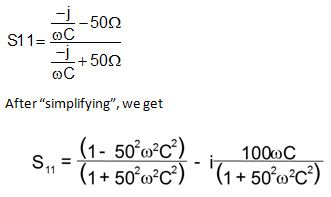
It’s hard to tell just looking at this, but if we pick one value for a capacitor, and plot S11 on a polar plot, as we sweep frequency, we get a very simple pattern. We can sort of figure it out.

Since there is no loss in an ideal capacitor, anything we send into it must come out. The magnitude of S11 must be 1. This means S11 on a polar plot must be along the outside edge of the circle. At low frequency, a capacitor looks like an open, so it must start on the right edge where an open lies. From looking at the analytical solution, as we increase frequency, we can tell the imaginary term will increase and the negative sign says the imaginary component will be an increasing negative value.

This suggests, the return loss, on a polar plot, will be on the unit circuit, starting at the far right and as we increase frequency, rotate in the clockwise direction.

Likewise, for an ideal inductor, we get S11 as:

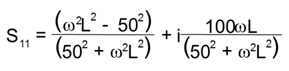
At low frequency, an ideal inductor is a short, so will start on the far left, be on the unit circuit and rotate clockwise as we increase frequency. These examples are shown in Figure 4.

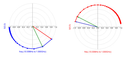
Figure 4. Examples of S11 on a polar plot for an ideal capacitor (left) and ideal inductor (right).

Now we see very specific patterns:

1. An open is a dot on the far right
2. A short is a dot on the far left
3. A resistor is a dot on the real axis
4. A capacitor is always on the unit circle in the lower hemisphere
5. An inductance is always on the unit circle in the upper hemisphere
6. A transmission line circles rotates around the unit circle

A Generalized Impedance

We can describe any impedance, at some frequency, as a real component and an imaginary component,

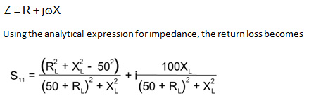
This looks so complicated! What insight can we possibly get from this equation?

Let’s look at the pattern of S11, for the case of a fixed resistance. In other words, let’s pick a value of resistance, R = 50 Ohms, for example, and sweep the reactance to be anything. It can only range from – infinity to + infinity. As we sweep the reactance, what will the pattern of S11 be?

Just looking at this relationship, I haven’t a clue. Other folks, much better at geometry than I am, could probably predict the pattern. Instead, I’m just going to use the power of simulation and calculate the S11 on a polar plot for this case, as we sweep the reactance. And then, I’m going to use a few other values of resistance and plot other S11 lines of constant resistance.

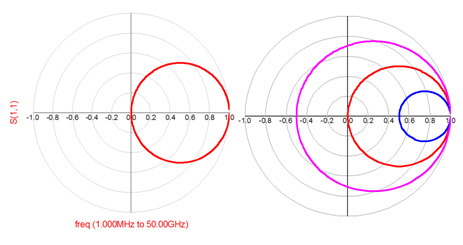
Figure 5. S11 plotted on a polar plot for the case of constant resistance and all possible reactances. Left, the case of R = 50 Ohms, right, the case for 25 Ohms, 50 Ohms and 75 Ohms. These are return loss lines of constant resistance.

It is remarkable that return loss lines of constant resistance are circles on the polar plot. If the return loss of any DUT were to lie on one of those circles, we could tell instantly what the real part of the impedance was, at that specific frequency.

In the same way, we can fix the reactance to one value and sweep he resistance from 0 to infinity. This would give us S11 lines of constant reactance. When the reactance is negative, such as form a capacitor, we expect S11 to always be in the lower hemisphere. When the reactance is positive, as with an inductor, we would expect the lines of constant reactance to be in the upper hemisphere. Examples of S11 lines of constant reactance are shown in Figure 6.

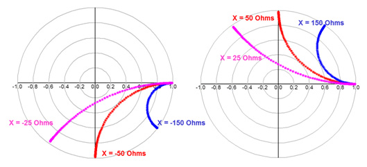
Figure 6. S11, plotted on a polar plot, for the case of constant reactance while sweeping the resistance. Left, three values of negative reactance and right, three values of positive reactance.

It is remarkable that for such complicated analytical equations for S11, the patterns S11 makes on a polar plot are simple. Lines of constant reactance are really great circles, either in the southern hemisphere or in the northern hemisphere.

These two sets of plots, for lines of constant resistance (the real part of the impedance) and lines of constant reactance (the imaginary part of the impedance), suggest that we can read right off the polar plot, the real and imaginary part of the impedance of any DUT from its S11, at any specific frequency.

Enter the Smith Chart

If we were to leave these values of S11 for constant real and imaginary components on the polar plot curves, we could use them as reference grid lines to read impedance right off the plot. That’s what a Smith Chart is. It is named after Phillip Smith, who created it while at Bell Labs in the early 1930’s.  An example of a Smith Chart is shown in figure 7.

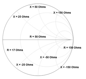
Figure 7 A Smith Chart which is a polar plot of S11 with lines of constant reactance and constant resistance superimposed.

When we plot S11 on a Smith Chart, we are really plotting S11 on a polar plot. It’s just that we added some extra grid lines and removed the polar plot grids.

While Smith Charts are valuable for rf engineers who care about the impedance of a structure at a specific frequency, they have much less value to a Signal Integrity engineer, who cares about the impedance of interconnects over a wide frequency range, and especially in the time domain.

Instead, the best way a Signal Integrity engineer can use the Smith Chart is by recognizing it is a polar plot of S11 and look for the overall patterns created by the measured or simulated return loss.  At a glance, we can identify features of the DUT by looking at the patterns.

The return loss of every DUT on a polar plot, or Smith Chart, has a distinctive pattern. Figure 8 shows an example of short transmission lines terminated with an open and a short and a surface mount 50 Ohm resistor.

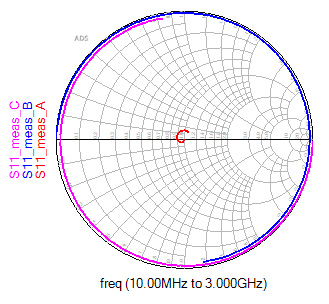
Figure 8. Smith chart plot of S11 for two transmission lines with an open and short termination and a 50 Ohm SMT resistor.

 Just at a glance, we can see the open transmission line starting at the open position, rotating in the clockwise direction looking like a capacitor, and continuing to the region of an inductor. Likewise, the transmission line with the short, starts at the short position, rotates in the clockwise orientation looking like an inductor and then begins to look like a capacitor.

The SMT resistor starts out looking like a 50 Ohm resistor, then spirals a little in the clockwise direction, looking initially like a capacitor, and then moves around to look like an inductor.

The next time you have a 1-port S-parameter to look at, don’t hesitate to display it on a Smith Chart, but think “reflected signal on a polar plot.”