Assessing the Accuracy of EM Simulation Tools

Electromagnetic simulation tools will almost always give a result for any problem after pressing the run button. But is the result accurate? A methodology is introduced to establish the best practices for using the Ansys 2D Extractor and HFSS tools that include recommendations for the setup conditions, balancing accuracy, and computation time. With this methodology, an error in the absolute accuracy when solving for some electrical features can be achieved to better than 0.3%. This methodology can be extended to other more complex structures and applied to other field solver tools. 

Methodology

When using a field solver tool for the first time, it is a best practice to simulate something for which you know the answer.^1,2,3 This way, you are able to apply Bogatin’s Rule #9: anticipate before you simulate.⁴

One interconnect figure of merit that is important to calculate with a field solver is the characteristic impedance of a uniform transmission line. The twin round rod is a structure that can be analytically solved exactly. The methodology presented here is for setting up a field solver tool and evaluating the characteristic impedance of a twin rod pair. An example of the typical structure simulated is shown in Figure 1.

Figure 1. An example of twin rod structure: two round cylinders with a fixed pitch.

The characteristic impedance of a twin rod has an exact analytical expression given by

where s is the pitch (center to center spacing), r is radius of each cylinder, and Dk is the relative permittivity of the medium completely surrounding it.

This analytically calculated characteristic impedance is a reference that can be used to verify the accuracy of any numerical simulation tool. In this article, this methodology is applied to exploring the Ansys 2D Extractor and HFSS full wave solver. This analysis applies equally well to the full version and the free student version.⁵

Setting Up the 2D Extractor

Once the geometry is created in the 2D Extractor and the signal and ground conductors are defined, the only parameter to adjust is the criterion for convergence. Every field solver tool will create a mesh in which Maxwell’s equations are approximated and solved. The accuracy of any tool is fundamentally related to the density of the mesh and how well the equations are approximated in each mesh element.

Typically, the more mesh elements there are, the longer the computation time, but the higher the accuracy. The Ansys 2D Extractor uses an adaptive mesh generator which optimizes the mesh so that each time it is refined, more mesh elements are created where there is the highest field gradient. This optimizes the number of mesh elements for accuracy and compute time.

For example, Figure 2 shows the mesh generated for the initial pass and for the fifth pass. The new mesh elements are created where the field gradient is highest. How many passes are enough?

Figure 2. Example of the mesh generated initially and after five passes.

The number of passes to refine the mesh can be set manually or automatically based on a convergence criterion labeled as delta energy. This term is the percentage change in total energy from the previous adaptive pass to the current pass, relative to the total energy calculated in the previous pass. The total energy is the integral of the energy in the electric field throughout the volume of the problem. As the mesh is refined, the total energy in the electric field will converge to a final value, and the change in each iteration will be smaller. 

While this is a useful metric of how close to a final answer each iteration might be, it is not clear how this relates to how close to a final value the characteristic impedance calculation might be. To establish the correlation between delta energy change and the final value of the characteristic impedance, a simple numerical experiment was performed. 

A twin rod structure was created in the Ansys 2D Extractor tool with air as the surrounding medium. The condition for mesh refinement on each pass was set as a maximum of 30% refinement, the default condition. Passes were iterated manually and after each mesh refinement pass, the characteristic impedance and the delta energy change were recorded. Figure 3 shows the value of the delta energy percent change and the percent difference in calculated characteristic impedance to the final value after pass 25. This is compared with a simple model assuming a 30% reduction in the change per pass.

Figure 3. Correlation between the characteristic impedance and delta energy convergence and a simple model of the error reduction reducing by 30% per pass.

This comparison illustrates that the delta energy percent change term in each pass closely matches the characteristic impedance convergence to the final value. This establishes confidence that the delta energy convergence value is a good surrogate for the convergence of the final value of other electrical metrics. It also suggests that the improvement in accuracy with each pass increases faster than just the maximum number of mesh elements.

To achieve a calculated value of characteristic impedance that is within 0.1% of the final value, the delta energy convergence should be set to a value of 0.05%.

Translating the Real Problem into the Tool Environment

The next step is deciding how to translate some of the features of the real structure into the 2D Extractor environment. A round structure is described in rectilinear geometry as a polygon with a finite number of facets. How many facets around the circumference are enough?

As a simple numerical experiment, the number of facets of each rod was increased and the characteristic impedance was calculated using the convergence criterion of 0.001% delta energy for each calculation. The difference in calculated characteristic impedance for each number of facets with the final value for more than 1500 facets was simulated as the number of facets increased. Figure 4 shows the reduction in the difference between the characteristic impedance and the final value. It is interesting to note that while the Ansys manual does not state the default number of facets used, it can easily be reverse engineered. The characteristic impedance value for the case of 70 facets matched the simulated impedance for the default setting. For a value within 0.1% of the final value, a total of 200 or more facets should be used.

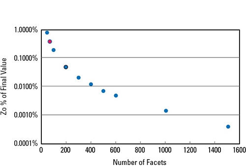
Figure 4. Impact on convergence of Z0 from number of facets for 50 Ω twin rods.

Absolute Accuracy of the 2D Extractor

Once the condition for convergence is established as well as the recommended number of facets, the next question is: what is the absolute accuracy of the 2D Extractor tool? 

Every simulation is always a balance between compute time and accuracy. In principle, if the numerical solution to Maxwell’s equations is implemented correctly, an arbitrary accuracy can be achieved with an arbitrarily fine mesh. We set a starting goal of an absolute accuracy of better than 0.1% error. This requires setting the convergence in the delta energy to 0.05% and the number of facets to 200.

The 2D Extractor uses the background as the extent of the space in which the fields are calculated. This is not a term that can be adjusted, and it is not clear from any documentation on the size of the region. To view the mesh or any calculated field quantities, a boundary region must be created. When this region is filled with air, there does not seem to be any impact on a calculated electrical parameter from the extent of this region. 

The analytically calculated impedance of the twin rod structure was 50.000 Ω, while the numerically calculated characteristic impedance was 50.009 Ω. They agree to within 0.02%. This is a direct confirmation of the absolute accuracy of the 2D Extractor tool.

Summary of Best Practices Using the 2D Extractor

Based on simple numerical experiments, a few general guidelines have been established to achieve an absolute accuracy in calculating the characteristic impedance of twin rods in the 2D Extractor tool:

1. Set the delta energy convergence to be lower than the absolute error required. For an error of 0.1%, set the delta energy convergence to 0.05%.
2. When translating a round structure into a faceted structure, use at least 200 facets for an absolute accuracy better than 0.1%.
3. When modeling a homogeneous infinite extent dielectric, change the Dk of the background to match it. When modeling localized dielectric regions, as a starting place, assume the electric fields extend 10x the pitch between conductors to achieve a value within 0.1% of the infinite extent case.

It is remarkable that the absolute accuracy of a numerical simulation can easily approach better than 0.1% error to an analytically exact case. This enables the use of the 2D Extractor as a reference to calculate the characteristic impedance of any arbitrary structure. This methodology and the results of the 2D Extractor are applied directly to establish the best practices for HFSS, a full wave 3D EM solver.

Setting Up HFSS

HFSS is a general, arbitrary, 3D full wave simulation tool. While it is a workhorse tool for antenna and radiated emissions problems, it is becoming a powerful tool to analyze interconnects for signal integrity applications.

When dealing with interconnects imported from circuit board layout structures, lumped ports are typically used. This is the case when there is a single conductor identified as the return path. Otherwise, when there are multiple return conductors and the interconnect structure begins and ends at a uniform transmission line cross section, a wave port is recommended. Lumped ports and a radiation boundary condition were exclusively used in all the problems presented in this article.

The twin rods problem was used to establish confidence in the results from HFSS. While it is the S-parameters of the structure from the lumped ports which are calculated, this was translated into a characteristic impedance by simulating an electrically long structure and using a TDR simulation of the return loss to extract a value of the characteristic impedance. Figure 5 shows an example of the twin rod structure, the simulated S-parameters, and the simulated TDR from S11.

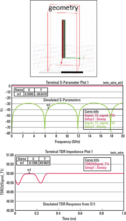
Figure 5. The process flow from the geometry to the extracted characteristic impedance. Note the impact of the lumped ports in this example is to add a small amount of excess capacitance to the ports.

In setting up the tool, there are a number of parameters to adjust. The methodology of starting with something for which you know the answer and comparing the analytically exact answer with the simulated result was applied to evaluate the best practices for:

• Criteria of delta S for convergence
• The size of the lumped port
• The minimum physical length of the structure to be electrically long and use TDR to get the characteristic impedance.

Convergence Criteria

The convergence criterion in HFSS is based on the largest change in any S-parameter with each iteration. Each iteration refines the mesh in regions in which there are large field gradients. The default maximum increase in mesh elements from pass to pass is 15%. Using the same methodology as with the 2D Extractor, the connection between the convergence in the delta S term and the extracted characteristic impedance can be correlated with the number of iterations. Figure 6 shows this connection.

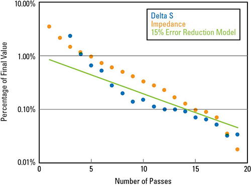
Figure 6. The percentage convergence to delta S per pass and the percentage of the impedance to the final impedance.

There is also a good correlation between the delta S condition and the convergence in the characteristic impedance of the twin rod. A convergence in the characteristic impedance to 0.1% of its final value requires a convergence of delta S to better than 0.1%. The correlation between the delta S and the absolute accuracy of the characteristic impedance is structure dependent and not precise. As a starting place, in the case of the twin rod geometry, for convergence in the characteristic impedance to within 0.1% of the final value, the delta S convergence criteria should be at least 50% smaller, or 0.05%. In this example, this required more than 15 passes.

This is based on a very specific geometry. It may vary with other geometries. For example, if the problem involved an electrically short structure, such as a via, in an otherwise large structure, the accuracy of recovering the S-parameters of the via structure may not be indicated with the overall delta S value. This suggests that an important practice is to keep the non-essential structures to a minimum length so they do not dominate the S-parameter convergence.

Number of Facets to Approximate Round Structures

When translating a round structure into a faceted structure in HFSS, it was found that 70 facets are required to get a convergence of 0.1% in characteristic impedance to the final value. The results of this analysis are shown in Figure 7. It is also interesting to note that the default condition in HFSS can be reverse engineered as 20 facets. This default condition results in a value that is only within 3% of the final value. 

Figure 7. The characteristic impedance converges to a final value as the number of facets increases.

The Size of the Lumped Port

The lumped port, using terminal mode, will connect between the signal and its return path. In the case of the twin rod, the lumped ports can be as small as the spacing between the twin rods or as large as the extent of the edges of the rods.

Using the conditions of 15 passes and 70 facets, the characteristic impedance was calculated for different lumped port sizes from the minimum dimension just touching the signal and return conductors together and overlapping them. The absolute accuracy of the calculated characteristic impedance did not depend on the lumped port size to within about 0.5% of the absolute accuracy. This result, shown in Figure 8, was limited in accuracy by the 15 passes used.

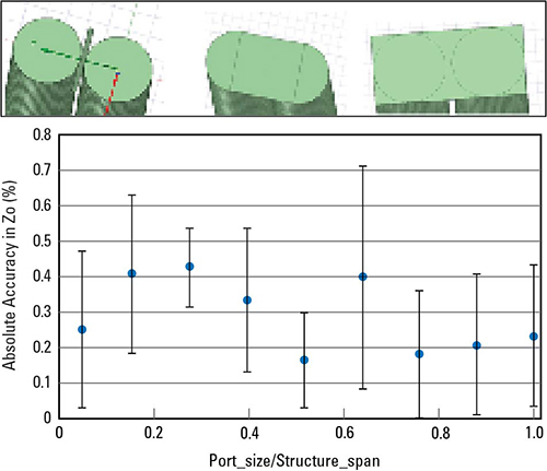
Figure 8. The extent of the lumped port (a few examples shown in the insert) has no impact on the absolute value of the characteristic impedance to within about 0.5%. The error bars represent the uncertainty in extracting the characteristic impedance from the TDR.

Electrically Long Structures

In order to use the TDR simulation to extract a value for the characteristic impedance of the twin rod structure, it must be electrically long. This way, the TDR profile will show a flat top or flat bottom from which the characteristic impedance can be interpreted from the constant instantaneous impedance.

This condition is usually based on the common rule of thumb, TD > ½ the rise time.⁶ This results in an estimate that the physical length should be larger than about ½ wavelength for the highest frequency used in the simulation. Longer than this physical length, the impedance should not depend on the electrical length.

In these simulations, to see a flat top or flat bottom with better than 0.1% uncertainty, we found that a more robust estimate is TD > rise time. This translates to the electrical length > the wavelength at the highest simulated frequency. This is illustrated in Figure 9.

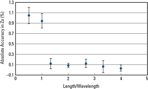
Figure 9. The absolute accuracy in the characteristic impedance as the electrical length is increased. A robust rule of thumb is that the length should be greater than the wavelength.

Summary of Best Practices Using HFSS

Based on a few simple numerical experiments using twin rod structures, some general guidelines have been established to achieve an error in the absolute accuracy in calculating the characteristic impedance in HFSS that is better than 0.3%.

This analysis used lumped ports for the structure under test. This is limited to the case when there is a connection to only one signal and one return conductor. As revealed in the TDR simulations, the lumped ports introduce a discrete excess impedance to the launches. This will ultimately limit the useful bandwidth for very accurate results. However, using TDR to extract the characteristic impedance of an electrically long, uniform transmission line effectively time gates this simulation artifact from the calculation of the characteristic impedance.

This analysis was based on a very special case which may not have a similar geometry to other problems, but it is a starting point to evaluate the process of setting up and using HFSS or other electromagnetic simulation tools.

A best practice when using a new tool is to always start by solving something for which you already know the answer. In this case, a twin rod geometry can be exactly solved analytically and used as a reference. After establishing a methodology of achieving better than 0.1% absolute error in the 2D Extractor tool, any arbitrary structure can be solved in this tool and used as a reference in an HFSS calculation.

There will always be a fundamental trade-off between the complexity of the structure, the absolute accuracy required, and the compute time and resources. The convergence criterion is one term to adjust this balance.

Only one electrical figure of merit, the characteristic impedance of the interconnect, was evaluated in this analysis. But this methodology can be applied to explore the best practices for other criteria, if you start with something for which you know the answer. 

The recommended best practice to achieve a level of absolute accuracy in HFSS is as follows:

1. Set the delta S convergence to be 50% lower than the absolute error required. For an error of 0.1%, set the delta S convergence to 0.05%, i.e. the value of delta S in simulation tool is 0.0006. For an error in the absolute value of 2%, use a value of 1%.
2. When translating a round structure into a faceted structure, use at least 70 facets for an absolute accuracy better than 0.1%.
3. The size of the lumped port is not important if it connects the signal and return conductors.
4. The extent of the radiation boundary is not important for calculating a characteristic impedance. It may be important if radiation effects are considered.
5. The minimum physical length of the structure, in order to be electrically long and use TDR to get the characteristic impedance, should be longer than the wavelength of the highest simulated frequency.
6. Be aware that the lumped port does add a small excess impedance to the launches.

REFERENCES

1. J. C. Rautio, “An Ultra-high Precision Benchmark for Validation of Planar Electromagnetic Analyses,” IEEE Transactions on Microwave Theory and Techniques, Vol. 42, No. 11, Nov. 1994, pp. 2046–2050, doi: 10.1109/22.330117.
2. J. C. Rautio, “Experimental Validation of Microwave Software,” ARFTG Conference Digest, 1990, pp. 58–68, doi: 10.1109/ARFTG.1990.323981.
3. K. Z. Aghabarati and L. E. Rickard Peterson, “Overview of the Iterative Solver in HFSS for Analysing Frequency Domain Electromagnetic Problems,” International Applied Computational Electromagnetics Society Symposium, 2019, pp. 1–2.
4. E. Bogatin, “Signal and Power Integrity-Simplified,” Prentice Hall, 2009.
5. Ansys for Students, https://www.ansys.com/academic/students.
6. E. Bogatin, “Bogatin’s Practical Guide to Transmission Line Design and Characterization for Signal Integrity Applications,” Artech House, 2019.