
As you know, "us", Signal and Power Integrity Engineers, are full of tricks, rules of thumb, and shortcuts. These tricks mostly help us understand something, save analysis time and, why not, make us look smarter than we really are!! In that vein, seldom have I encountered a quick and dirty trick as useful and underestimated as S-parameter renormalization.
Perhaps you are working in the frequency domain, and need to answer a simple set of questions that would be more natural to answer in the time domain. Or, maybe you are trying to determine, at a high level, how things would work if a termination here and there had to change, or maybe you really, really want to cheat and see what would happen with that perky connector, if one of the pins was connected to ground instead of to a signal. In many of these cases, the simple trick of renormalization can give you a quick answer and it will provide insight into the underlying structure to analyze.
Before we start, let me very briefly review the fundamentals of S-parameters mainly to highlight where the renormalization impedance fits in the whole picture.

Let’s imagine we inject a normalized voltage wave (a1) as shown in Figure 1, traveling from source (left termination) to the DUT [S] through a connecting cable with characteristic impedance (Zc). When the wave arrives at the interface between the DUT and the cable, it will either be reflected as (b1) or transmitted at the other side of the DUT as (b2) or a combination of both. The wave (b2) coming out of the DUT on the right, will propagate all the way to the end (right termination). The same thing happens if the injection point is on the right. Just reverse the 1s by 2s in the above description.
S-parameters are the ratio of reflected to incident waves at points 'D' for matched conditions at points ‘C’. Important to pause a moment and realize that the location of the matching condition (point C) is NOT the same as the location where the S-parameters (ratio of waves) are calculated (point D). The matching conditions are formally expressed as a1=0 and a2=0 as shown in Figure 1
It's all about reflections (or the lack thereof), in order to extract S-parameters, we can't have reflections at point "C", as shown by the condition a1,a2=0, but the key here, is to realize you can reflect to your heart's content at point "D". I find this simple point to be a source of confusion to S-parameters newcomers. In essence there can be none, or a lot of reflections at the interface point between the DUT (the thing you want to measure) and the instrumentation setup (cables used to connect your instruments to the DUT).
The next point to realize is that the amount of reflections at ‘D’ will directly depend of the DUT characteristics (input/output impedance) and the instrumentation, or what I call, "renormalization" impedance. In this simple example you can envision the renormalization impedance to be the Zc of the cables connecting to the DUT and the end terminations, (for example and in general 50 Ohms).
Just to stress this point, let's say in Figure 2 (left) a measurement is taken of a uniform and homogeneous, lossy and causal transmission line with a Characteristic Impedance (Zc) of 50 Ohms. As you can see, these S-Parameters would make any SI engineer drool, with smooth decaying insertion loss (IL), and very little return loss (RL=-45dB).
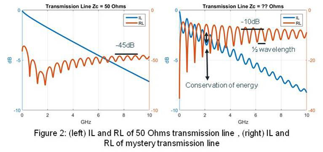
You might be wondering: If the transmission line is so perfectly matched, why the return loss is not -∞? The answer is that nothing is perfect in life. A real lossy, causal and passive line will have a complex characteristic impedance (Zc) not identical to the real renormalization impedance (50 Ohms in this case) and furthermore the line impedance will change over frequency, these two things will generate an small amount of reflections resulting in a finite return loss. You should only expect a -∞ return loss for an ideal lossless and frequency independent transmission lines case.
But if I were to ask you, what on earth was measured on Figure 2 (right) ?, you might be quick to answer, certainly not a 50 Ohms transmission line, since there are more wiggles (SI terminology) in the IL and much higher RL=-10dB.
Even though the answer would make perfect logical sense, in this case, it would be incorrect. Actually the exact same Zc = 50 Ohms transmission line as shown on Figure 2 (left) was measured, but the "renormalization impedance" used, was changed to 25 Ohms, tricky me!!!
And here is another key of S-parameters, often times neglected and forgotten by newcomers. S-parameters by themselves are incomplete if not provided with its instrumentation impedance. You can think of the renormalization impedance as the Jerry Maguire "you complete me"[1], of S-parameters.
Before we move on, I’ll digress just a little bit and highlight a couple of interesting points in Figure 2:
- Note, how on the very reflective case, the IL oscillates. When the IL goes down, the RL goes up and vice-versa. As our forefathers predicted, energy is not lost, but transformed. This means that the energy not transmitted, is either dissipated (heat) or reflected. By observing S11 (reflection) and S21 (transmission) on the same plot, we can clearly see, a high in S11 (more reflections), results in a low in S21 (less transmission). Of course this can't be easily observed in Figure 2 (left) since in this case, the transmission line is very well matched to the renormalization impedance of 50 Ohms and reflections are finite but very small.
- Also note the nice periodicity of the oscillation. This is produced by the ½ wave resonance of the structure. Transmission line terminated with the same reflective impedance at both ends.
Ultimately, the point is that the S-parameters results you see on Figure 2, for the SAME underlying structure (DUT) dramatically depended of the renormalization impedance.
Now, if you are inclined to, or maybe after a drink or two, or … three, you can take this concept to the extreme, for example by renormalizing the S-parameters at every single frequency point with different complex renormalization impedance. This technique has proven to be very useful in many cases, and there are a few Design-Con papers to prove it [2], but it’s outside the scope of our simple cheating discussion.
But even for the simple case of manipulating the S-parameters by renormalization with single real impedance at all frequencies, we can still quickly observe interesting structural behaviors.
Let's say, for example, someone drops an S-parameter touchtone file on your desk and asks for your opinion.
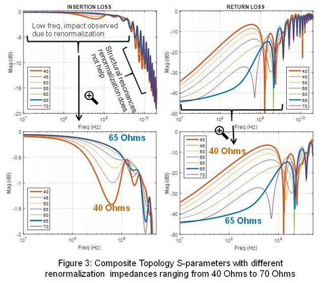
You plot it (Figure 3) and realize the insertion loss has those annoying periodical wiggles at low frequencies, and you immediately say: "hmmm, maybe this line is not 50 Ohms". You decide to renormalize the S-parameters to various impedances and you see that at lower frequencies, less than 2GHz, a renormalization impedance of 65 Ohms provides the best return and insertion loss, then after 2GHz there is not much improvement, if any.
Since you don’t trust anything yet, and have ample time to spare, you decide to calculate and plot the TDR of the structure (Figure 4).
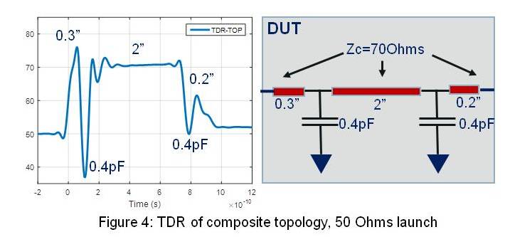
The topology contains three sections of transmission lines separated by capacitors representing via loading (Figure 4, right). The impedance of all three lines is 70 Ohms, and the caps are loading it down. The topology in the example is known because I created it, but often times, that is not the case, and then, is when TDR comes to our rescue (Figure 4, left).
As the signal propagates through the topology it losses energy and TDR resolution starts to degrade as evidenced by the second capacitor dip, but overall, the spatial resolution (not readily seen in the frequency domain) of the TDR provides a clear picture of the topology and that is why "we SI guys", love it so much.
Perhaps this application only requires you to pass data through this topology at 3GHz (6GB/s) or less and you decide it'll be good to understand how to correlate the time domain TDR measurement to the frequency domain S-parameters shown in Figure 3
When you embark on the analysis, you fundamentally observe two features:
- Renormalizing the S-parameters to 65 Ohms (almost 70 Ohms) provides the best IL and RL at frequencies bellow 3GHz.
- Above 3GHz there are stable oscillations in the structure that renormalization can't help with
Both of these observations can be explained by the structural resonances of the circuit formed by the boundaries of impedance discontinuities between features, for example, to list a few:
- Between the beginning and end of the DUT the renormalization impedance (50 Ohms) at both ends is different than the Zin and Zout of the DUT. The length of the DUT is around 600ps as seen on the TDR. Since terminations are the same at both ends, we know the structure will resonate as a ½ wave resonator, hence Fr = ½ *1/600ps = 833MHz. We can clearly see a dip on IL and a peak on RL at that frequency for the mismatched case. We also notice that for the case when we change the renorm-impedance to 65 Ohms or 70 Ohms the low frequency peak (833MHz) goes away.
- Between vias, approximately 350ps distance apart (same via impedance, hence ½ resonance), and a resonance frequency of Fr = ½*1/350ps = 1.42GHz, as also seen on the S-parameters of Figure 3
In order to visualize better why a 70 Ohms renormalization impedance gets rid of the low frequency resonance, lets plot a TDR using a 70 Ohms launch (at both ends) as shown in Figure 5. In this case the low frequency resonance goes away as shown in the S-parameters and also as seen on the TDR. By launching with 70 Ohms we are minimizing the discontinuities at the entry and exit points of the DUT, thus improving the S-parameters IL and RL at those frequencies.
We are still left with the resonant structure generated by the separation between vias (caps) and, short of improving the via/reducing capacitance, there is no much else we can do with renormalization impedance.
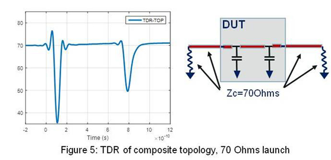
Bottom line, when inserting this small DUT block on a larger structure, you know that a target system impedance for that larger structure of 70 Ohms will improve the overall behavior (particularly below 3GHz).
Just to keep your juices going, let's look at another application where renormalization tricks can prove to be very useful, for example on coupled structures, (connectors, group of vias, transmission lines etc).
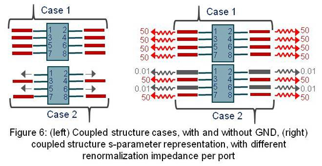
In the following example I have created a coupled 8 port DUT and, for the purpose of this discussion, let's assume it is a connector. We would like to try different pin-outs patterns, including different ground configurations.
There is another minor twist we need to internalize before we can understand the following example. In general, with multiport S-parameters, we use the same renormalization impedance at all ports. Even though this is very convenient, it's not necessary. Every port could have its own different renormalization impedance
Figure 6 (left) shows just two what-if scenarios I would like to explore. Case-1 is where the connector is fully utilized, and all the ports are used for signals. Case-2 is where we want to explore what would happen if we connect a couple of pins to ground.
To do this directly in the S-parameter world, without anything else, as long as we have a viewer or script that can perform independent impedance port renormalization, the problem is trivial.
The right side of Figure 6, shows how we would have to set our renormalization impedance for each port on both cases, and the left is what that means when we insert the DUT in the system.
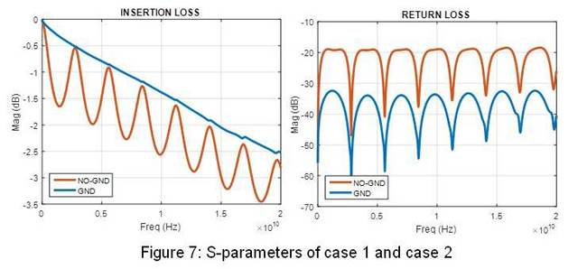
Just doing renormalization and plotting S43(IL) and S33(RL) as sown in Figure 7 exposes a big difference between these two cases. Case-1 seems very mismatched while case-2 looks much closer to 50 Ohms as can be directly seen in the frequency domain. At this point it's easy for us to recognize the periodical oscillations of the structure and realize there is no other structural resonance other than the end-to-end ½ wave resonance between DUT and renormalization impedance miss-match.
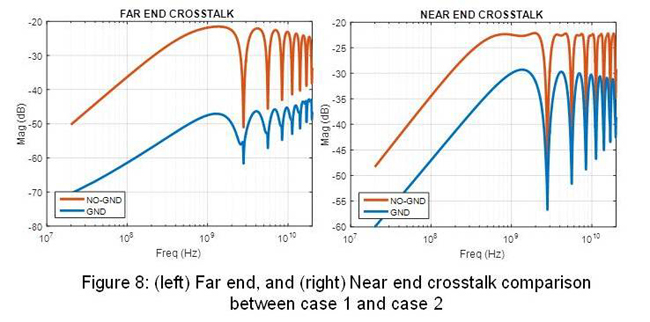
We can of course compare the difference in crosstalk from port 3-4 to port 7-8 for example, as seen in Figure 8, and in this case, we see a big improvement when GND are added.
As shown in the previous examples, doing quick and dirty renormalization tricks with S-parameters can not only save some time in certain cases, but also, when coupled with TDR, aid in the understanding of the underlying structures by helping with correlation between frequency and time domains.
Now, remember the title of this article has two words: cheat and art. The art, when cheating, is to know the things you might be neglecting or purposively overlooking, and targeting just the information you are really after.
Now that you have this other tool in your toolset, likely you'll find many other uses for it that might help with your day to day work. After you master this, If you find yourself a Friday afternoon trying to get something done but you are eager to get back home or perhaps watch the latest episode of Game of Thrones, regardless of the bla,bla,bla,TDR,bla,bla,bla,ABCD,bla..etc things what your geeky colleagues with thick glasses might tell you, with confidence, cheat.
Bio:
 Gustavo J. Blando is a Senior Principal Hardware Engineer with over twenty years of experience in the industry. Currently at Oracle Corporation, he is leading the SI/PI team and responsible for the development of new processes and methodologies in the areas of broadband measurement, high speed modeling and system simulations. He received his M.S. from Northeastern University.
References:
[1]. Famous movie: https://en.wikipedia.org/wiki/Jerry_Maguire
[2]. Practical identification of dispersive dielectric models with generalized modal S-parameters for analysis of interconnects in 6-100 Gb/s applications, Yuriy Shlepnev