IPC 2152 [1], published in 2009, was the most thorough, most complete study of trace current/temperature relationships ever undertaken. It contains over 90 pages and charts looking at the relationships from numerous directions. Prior to IPC 2152, the industry had been using a set of charts that go back to an NBS document (Report # 4283) published in 1956 [2]. Apparently, the charts were first published as a part of a military standard, MIL-STD-1495, in 1973. They were later published in a subsequent series of standards, culminating in a MIL-STD-275E, published in 1984. Later still, the charts were published as part of an IPC standard IPC-D-275, and finally in IPC standard 2221A in 2003.

One of the most interesting findings in IPC 2152, compared to the earlier charts, is that internal traces are cooler that external ones for the same size and current. In the earlier charts, independent experimentation was not done on internal traces. Internal traces were just assumed to be hotter than external traces, and the external trace data were derated by 50% in accordance with that assumption.

Traces are heated by I²R heating. They are cooled by a combination of conduction through the dielectric, convection through the air, and radiation. It had previously been assumed that convection and radiation cooled the traces more efficiently than did conduction through the dielectric. Hence the assumption that internal traces were hotter than their external trace counterparts. It turns out that dielectrics, in fact, cool traces more efficiently than does convection + radiation, and therefore internal traces are relatively cooler [3].

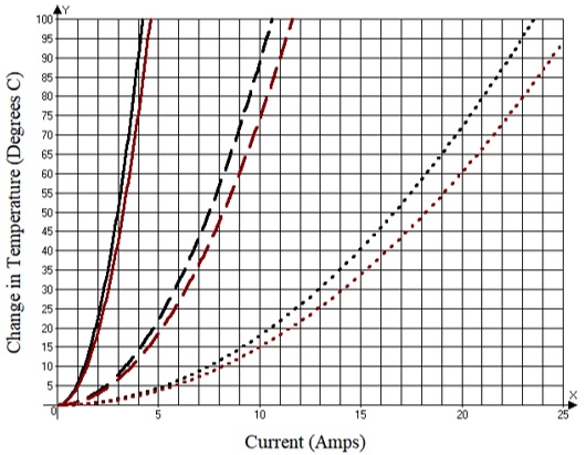
Figure 1 illustrates this relationship. It shows the current/temperature relationship for three different widths of 2 Oz. traces. Graphs of other trace thicknesses show similar results. Internal traces are cooler everywhere.

The following procedure was followed. Using the tables in IPC 2152, a sample of 44 data points was taken over three different trace thicknesses, 1.0, 2.0, and 3.0 ounces, several different widths for each thickness, and several different current levels. The IPC 2152 data and curves deal with temperature changes from ambient. Each data point included both internal and external trace temperature changes for otherwise identical trace/current combinations. The data were compared, and the relationship between the two changes in temperature (DTi vs DTe) was found to be much more complicated than first assumed. A regression analysis [5] was performed with the following resulting equation (Equation 1).

Eq 1.      

Where: DTi  = Change in temperature, internal trace, degrees C

The results illustrate that there is indeed “a predictable relationship between the external temperature of a trace and the internal temperature of the same trace carrying the same current.”

Since Equation 1 is non-linear and involves wide ranges in the values of the variables, it is difficult to represent it graphically and to draw any conclusions from it. But we can “normalize” it by dividing through by DTe. That gives us the ratio, DTi/DTe, which is more intuitively useful. Doing so results in Equation 2.

Eq 2.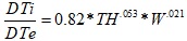       

Examining Equation 2, we can determine a couple of relationships:

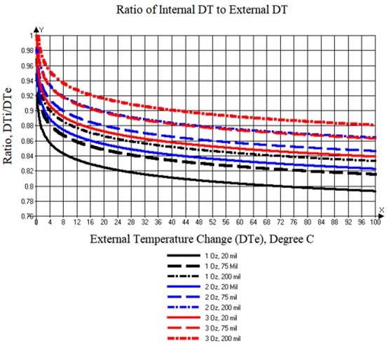
1. The ratio of internal change of temperature to external change of temperature decreases with increasing external trace temperatures, all other things equal. That is, internal and external temperature changes are relatively small at lower temperature changes. But internal traces get relatively cooler as (external) temperatures increase. This is because internal traces cool more efficiently than external traces do.

2. Thinner (internal) traces cool more efficiently than do thicker traces, all other things equal.

3. Wider (internal) traces cool more efficiently than do narrower traces, all other things equal.

The reason for these last two effects is that wider and/or thinner traces have relatively more surface area in contact with the dialect and therefore conduct heat away from the trace more efficiently. These three relationships can be seen in Figure 2.

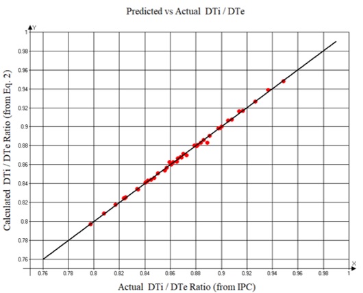
If we want to compare Equation 2 with the actual ratio of the temperature change as derived from IPC 2152, we can calculate the ratio of the temperature changes for each data point using Equation 2 for the analysis. Then, we can graphically compare this calculated result with that data point derived from the IPC 2152 actual curves themselves. We would expect the comparisons to be (approximately) equal. Figure 3 illustrates the result. It graphs the predicted vs actual ratio of the change of temperature, DT(internal)/DT(external), for each of the 44 data points of the sample. A 45-degree line is superimposed on the graph. If the predictions were perfect, they would all lay exactly on this 45-degree line. As can be seen, the fit is very tight.

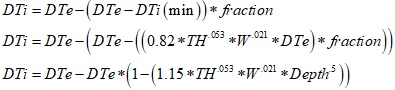
The results herein apply for internal traces in the middle of the board. Another question is, “What happens to the relationship for traces closer to an outside layer (i.e. not in the middle of the board)?” For any given trace configuration and current, the change in temperature will be a maximum for a trace on the surface of the board, and a minimum (DTi(min)) for a trace at the center of the board. (DTi(min) is what results from Equation 1. Therefore, the difference between the external and internal temperature change (DTe – DTi) is greatest at the middle of the board where DTi is at its minimum (DTi(min)), and lessens somewhat as the internal trace gets closer to the external layers. Modeling we have done with the software simulation tool Thermal Risk Management (TRM) [6] suggests that the cooling effect internal to the board kicks in at very shallow depths. We can define a term fraction to be the ratio of the difference between DTe – DTi at any depth to the maximum difference between DTe and DTi(min) at the midpoint of the board (Equation 3).

Equation 3:      Fraction = (DTe - DTi)/(DTe – Dti(min))

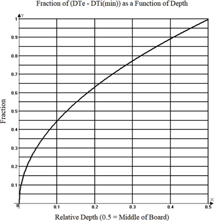
Fraction ranges from 1.0 at the midpoint of the board to 0.0 on the surface layer.  We estimate the relationship to be that shown as Equation 4 and plotted in Figure 4.

Equation 4:         

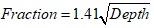
Where: Depth = the depth of the trace expressed as a fraction of the total board depth.

Figure 4 illustrates this. At a relative depth of 0.5 (middle of the board) the ratio of the internal temperature change to the external temperature change is 100% (1.0) of the result predicted from Equation 2 above. But let’s say a trace is at a relative depth of 0.1 (that would be just 6 mils into a 60 mil thick board). At that point the difference in trace temperatures would be 42.5% of the maximum difference, DTe - DTi(min).

As an example, let’s assume a 60 mil thick FR4 board with 20 mil wide, 1.0 Oz traces on the top layer and at the middle of the board. If the external trace is carrying 2.8 Amps, we might find that the external change of temperature is 40 degrees C. We can calculate the internal change in temperature, DTi, from Equation 1 or from Figure 2. Using Figure 2, we can calculate the internal change of temperature at the midpoint of the board, DTi(min), as 40 x 0.81 = 32.4 degrees C. That is 7.6 degrees C cooler than the external change of temperature. Now if the trace is 12 mils below the surface (instead of the middle of the board), i.e. the trace is at a depth of 12/60 = 0.2, then, from Figure 4, the difference between the internal temperature and external temperature changes would only be 0.63 times that just calculated, or 0.63 x 7.6 = 4.8 degrees. The internal change of temperature, DTi, would be 35.2 (i.e. 40 – 4.8) degrees C (a few degrees hotter than at the midpoint), but still cooler than the external trace.

 

There are a few caveats to this analysis. As we point out in our book [3] and in a previous article [6], one of the most important determinants of trace temperature is the thermal conductivity coefficients of the dielectric. There are two such coefficients: one in the “in plane” orientation (parallel to the traces), and one in the “through plane” orientation (perpendicular to the traces.) These coefficients relate to the cooling efficiency of the dielectric, and the trace temperature is heavily dependent on them. The problem is, most material suppliers do not specify a thermal conductivity coefficient for their product offerings, and if they do, they typically offer only one value without specifying which coefficient it is. You probably cannot know the coefficients for the materials you are using, and IPC 2152 does not report the applicable coefficients for their measurements. So we can be comfortable that the above analyses apply pretty well to the IPC 2152 data (since that’s where our analyses were derived from), it is less clear how well they will apply to your particular boards and designs. (In fact, this is what our book [3] is all about.)

This article originally appeared in“Design007 Magazine”, Nov. 2018, p. 52, http://iconnect007.uberflip.com/i/1053050-design007-nov2018/52. It has been edited and is reprinted here with permission.
 

Notes: