Efficient Sensitivity-Aware Assessment of High-Speed Links Using PCE and the Implications for COM

Previous studies showed that the width of striplines and the dielectric permittivity predominantly impact the extracted S-parameters [3]. The same design variables are used in [21] without additional explanation. It is assumed that the authors likewise focused on the most relevant parameters. This study includes both parameters from a designers perspective, i.e., the width of the striplines is considered by means of the differential routing impedance.

The design space outlined in Table 2 is illustrated by means of differential transmission and reflection in the considered frequency range from 50 MHz to 40 GHz in Figures 7 and 8, respectively. The latter presents the PCE mean and 90% confidence interval. The second order PCE model (P = 2) shows a good to very good correlation with MCS. Deviations are observed near 33 GHz. These point to super-linear parameter dependencies that may require a higher order PCE model and more Monte Carlo samples near this frequency. 

Considering that only 1000 Monte Carlo samples were used, this is a very good overall correlation. Furthermore, the following study focuses on 100GBASE-KR4 with a Nyquist frequency of 12.9 GHz well below 33 GHz.

The result seems similar to the study of [3]. Indeed they validate the previously reported results. Note, however, that we choose a more general approach with this framework. The augmented network parameters presented in [3] yield the S-parameter as final and only result. The algorithm presented therein does not allow for further processing such as COM analysis. Figure 4 illustrates the proposed, more general approach and how different quantities can be derived using the same framework. Typically there exists no trivial mapping between the derived stochastic quantities such as .

Correlation and Validation of Uncertainty Quantification Methods

Prior to exploring the capabilities of PCE modeling, this section investigates the accuracy and computational costs of PCE in comparison to conventional modeling and sampling schemes. Preference and feasibility of methods are ultimately governed by the stochastic and statistical quantities of interest as well as accuracy requirements. Hence, special focus is put on these aspects. 

Minimizing implementation effort and computational cost is considered to be a secondary constraint. The implementation effort of a PCE framework is more considerable than that of a conventional DoE/RSM which relies on a robust regression algorithm. Building on the available open-source implementation of PCE utility algorithms, our framework eliminates this difference. Henceforth, PCE with or without ST can be used with similar little effort as a conventional DoE/RSM.

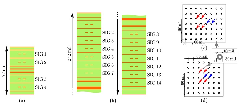
Figure 6: The link outlined in Figure 5(a) comprises two blades, two connectors, and a backplane. The stackup of the blades (a) features 14 layers, four of which are used for signal routing. The stackup of the backplane (b) features 38 layers, including 14 signal layers. Thicknesses are given in mil. The via pin fields near Tx/Rx SerDes and connector are given in subfigures (c) and (d), respectively. The differential pins of the victim are indicated in blue, two FEXT aggressors are indicated in red.

Figure 7:  Representative selection of 10 Monte Carlo realizations of the channel with N = 9 input variables. (a) Differential transmission (IL), (b) differential reflection (RL) are mostly well within the respective informative limit.

Figure 8: Mean (black) and 90% confidence interval (red/blue) of differential transmission and reflection of the high-speed interconnect with N = 9 input variables. Validity of results is confirmed using 1000 Monte Carlo samples. Losses are mostly well within the respective informative limit. The legends apply to both plots, respectively.

We propose the modeling flow depicted in Figure 9. Sampling schemes and surrogate models are implemented in a modular fashion. Note that obtaining the samples determines the overall computation cost for variability analysis of typical problems. Solving the linear system of equations for PCE and performing a polynomial regression fit for RSM come at practically no cost. Starting out with ST samples, both surrogate models can be constructed to yield stochastic and statistical insight into a black-box system as shown in Figure 9. Moreover, the models can be validated against each other.

If needed, more samples may be added to the RSM to improve the per-sampling accuracy. Note, however, that only PCE provides stochastic quantities as primary output. In the following, we use different combinations of sampling schemes as well as RSM to validate the PCE model where applicable.

The yield, measured by FPM, is one main concern in HVM production. It can be obtained from all three methods listed in Table 3 and merely requires a binning of samples in order to derive the underlying PDF and cumulative distribution function (CDF). MCS demands a high number of samples to achieve good accuracy. Even though the total number of link samples was limited to  = 1000 in this study, evaluation of the model takes more than 9 days.

Mathematical methods yield surrogate models, e.g., polynomials, from a reduced number of samples. In a second step, the same information as before is obtained in a matter of a few seconds by applying MCS to the surrogate model. In this study, PCE/ST and RSM with Box-Behnken (BB) sampling [22] (RSM/BB) both proved to be two orders of magnitude faster than MCS. Furthermore, both sampling schemes are based on a structured grid.

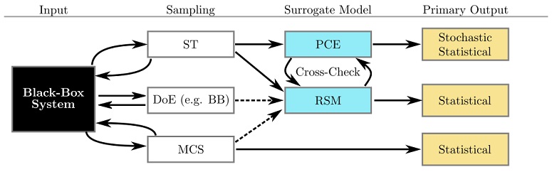
Figure 9: Combining PCE and RSM comes at practically no cost and increases certainty in modeling. The samples obtained from ST are fed into PCE and RSM. The former reveals important stochastic information such as relative impact and sensitivities at no additional cost. The per-sample accuracy of the RSM can be improved iteratively using samples from DoE or MCS. Additionally, some quantities may be obtained directly from MCS for validation purposes.

Table 3: Computation times for the analysis of 9 stochastically independent variables with 3996 frequency samples in the range from 50 MHz to 40 GHz each. Simulations are performed on a workstation with 32 GByte and 10 Intel(R) Core(TM) i7-4930K CPUs at 3.40 GHz in parallel. The total runtime is governed by  with 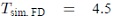  min per frequency-domain (FD) simulation of a component,  for concatenation, and  per statistical time-domain (TD) simulation.

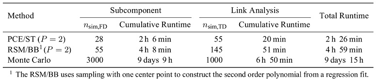
In classical segmented link analysis, this can be exploited to reduce the number of simulations. Figure 5c gives an account of the number of simulations per component. This benefit depends on the number of stochastically independent variables per subcomponent. Nevertheless, the full number of  simulations has to be performed for the time-domain analysis. Note how PCE/ST requires two to three times less samples than RSM/BB for a given approximation order of P = 2. For a non-segmented link simulation, the ratio would be equal to .

In the following, the constructed polynomials are compared by their ability to reproduce IL and COM by means of four statistical methods:

• The actual versus predicted comparison in Figure 10 gives insight into the per-sample accuracy of the model. Table 4 summarizes the root-mean-square deviation with regard to these plots in the first two rows. Excellent agreement is observed for both models for the IL. Good to very good agreement is observed for the COM values. The primary focus for ST is to use as few samples as possible to get the best stochastic approximation. This explains why the deviation from the training set is equal to zero for when using ST, because the 55 samples match the 55 degrees of freedom.
• The probability density function (PDF) is obtained by binning of Monte Carlo samples. The computational effort for this is determined by the time per function evaluation, i.e., simulation. Typically, several thousand samples are required for a very good convergence. Excellent agreement is observed for the correlation of IL models in Figure 11a. The fair agreement of PDF for COM in Figure 11d is assumed to be due to non-linearities in the COM implementation. For the purpose of this general design space study, this is a very good agreement.
• The cumulative distribution function (CDF) can be obtained from the PDF by integration. The value of CDF specifies the probability of a sample to lie in the interval . Hence, numbers relevant in production such as " % of yield has COM < 3" can be read directly from this curve. An application in the following section demonstrates this. Very good to good agreement of PCE, RSM, and MCS is observed for IL and COM in Figures11b and 11e, respectively.
• Confidence intervals (or percentiles) specify the range which guarantees to hold a given percentage of all possible samples. Compliance of a product may determine the lower bound of an acceptable COM value. On the other hand, an upper bound may be considered to avoid over-engineering. The agreement of confidence intervals in Figures 11c and 11f is very good to good with PCE being slightly pessimistic in predicting COM values.

Table 4: Root-mean-square deviation  of uncertainty quantification methods with N = 9 independent variables for selected metrics. The deviations are obtained by comparison with 1000 Monte Carlo samples.

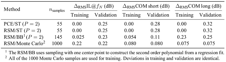
Figure 10: Predicted IL and COM values versus actual 100 Monte Carlo samples for (a—d) Polynomial Chaos Expansion (PCE) model with ST sampling and (e—h) Response Surface Method (RSM) with Box-Behnken (BB) sampling, respectively.

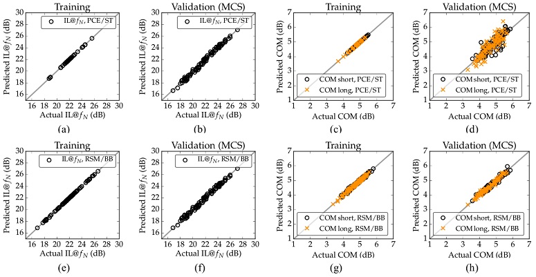
Figure 11: The correlation of the second order PCE/ST model and DoE/RSM reveals excellent agreement in case of  for all of the statistical measures (a) PDF, (b) CDF, and (c) 90% confidence intervals. Good to fair agreement is observed in for the analysis of COM by means of (d) PDF, (e) CDF, and (f) confidence intervals. Note that PCE gives a continuously pessimistic perspective on COM.

The number of samples used in constructing a polynomial model is a strong indicator for how much information of the parameter space is being used, i.e., the accuracy of a model. The RSM/BB seems to be closer correlated with MCS in some cases, but it uses almost three times as much information as PCE/ST.

For a fair comparison and for further investigation of this aspect, a RSM is constructed with the 55 PCE/ST samples. As Table 4 shows, the per-sample accuracy of this model is lower than the RSM that is constructed using 145 BB samples. Expectedly, it shows the same deviations from actual values that the corresponding PCE/ST model. This is because the polynomial regression in RSM degenerates to solving the same system of equations that is used to obtain the PCE model. On the other hand, constructing the PCE model from a larger number of samples is expected to yield even higher accuracy. In fact, constructing a RSM from 1000 Monte Carlo samples shows improved accuracy.

Sensitivity-Aware Performance Metrics and Applications

One of PCE's primary strengths is the ability to intrinsically assess the global impact of all considered parameters. The resulting Sobol indices of equation (7) are a measure for the relative impact of uncertainties across the entire design space. Based on the proposed framework, we demonstrate an in-depth compliance check of the previously studied 100GBASE-KR4 backplane link in this section.

Without further computational effort, the Sobol indices in Figure 12 reveal that the dielectric is the most influential parameter in the considered design space. In fact, it dominates the transmission as well as both COM cases. Its negative sensitivity with  means that the derivative  indicates a decreasing transmission as tan  increases. On the contrary, the connector quality factor  shows a positive sensitivity. As Q_C increases, the detrimental resonance frequency  moves further away from . Consequently, the transmission improves.

While COM is defined as the ratio of a signal to a noise figure, it shows similar trends as the transmission at the fundamental frequency of transmission. Note that the package termination impedance R_d is considered only in the COM algorithm. Hence,  shows zero sensitivity with regard to this parameter.

Previously, statistical quantities were derived with regard to the entire design space. Figure 12 reveals the dielectric of the backplane to dominate the design space. To determine whether a high-quality dielectric suffices to ensure a 3 dB COM margin, the dependency with regard to this parameter is further investigated.

Figure 12: The PCE model provides (a) Sobol indices that indicate the relative impact and (b) sensitivities of input uncertainty. The dielectric loss of the backplane dominates both  and COM in the design space and is further investigated as a primary design parameter. The IL is plotted as channel transmission  for ease of comparison. The legend applies to both plots.

It is coupled with the backplane  to mimic available materials, e.g.,  = 3.4 corresponds to tan  = 0.005. The joint CDF of the remaining seven parameters is obtained from Monte Carlo samples of the surrogate model.

Figures 13a and 13b show its dependency with regard to the backplane dielectric.  Note that a typical office computer completes this task within seconds. Figure 13c illustrates how the CDF is linked directly with the parts per million (ppm) fail rate, also known as failures per million (FPM). Considering the comprehensive design space at hand, the models show a good correlation. It can be seen that choosing a low-loss material with a tan  is beneficial to compliance of the link at hand. It sufficiently increases the COM margin so that the variation of all other parameters no longer violates the 3 dB margin.

Resolving a compliance challenge may not always be straightforward as depicted in Figure 13. The PCE model immediately provides information for a more detailed assessment of the relevant design alternatives. The relative impact may be plotted versus one or more design parameters. Figure 14 illustrates this for transmission , COM short, and COM long. Note that these plots need to be read carefully. They reveal relative impact, that is, trends that do not seem intuitive at first sight may be overshadowed by other effects. Moreover, the sensitivity trends depicted in Figures 14d through 14f do not resemble the information that is typically obtained from profilers. Instead, these plots show the evolution of the respective sensitivities as the backplane dielectric changes.

Figures 14a and 14d can be understood considering the model of a lossy transmission line which the interconnect essentially resembles at . The dielectric loss scales linearly with the frequency and the geometrical length. Hence, its impact on the overall uncertainty of  is largest through the 12 inch backplane. Changing the losses in the backplane raises or lowers the dB level, but does not notably impact the dependency of other parameters. Excluding it from the comparison reveals the dielectric loss in the 5 inch blade to be the second most influential parameter.

Furthermore, the backplane skew effectively degrades the differential transmission as discussed in [23]. A corresponding investigation of COM reveals how this performance metric is more comprehensive than the informative review of the IL. The time-domain analysis considers a wide frequency range and shows a higher relative dependency with regard to the connector as well as the package termination impedance R_d, both of which cause reflections.

Increasing the backplane loss (left to right in 14b) attenuates these reflections, effectively increasing the equalized signal amplitude . At the same time, the signal is attenuated which increases the impact of the blade dielectric.

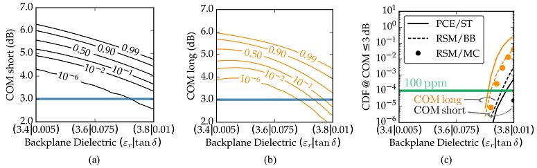
Figure 13: Plotting the partial CDF for a (a) short and (b) long COM package model versus the backplane dielectric visualizes how high-end materials ensure a low failure rate. Typically, a longer package transmission line leads to a lower COM. The observed CDF values at a fail/pass threshold of 3 dB are assembled in (c). Note that the CDF directly correlates with the failure rate, e.g., 100 ppm.A good correlation is observed for PCE and RSM. MCS results are not available due to the limited number of 1000 samples across the entire design space. The sampling range was limited to the interpolated design space (77% of total range) for a fair comparison of the polynomial models.

While not shown, a comparison of the Sobol indices for  and  reveals that the variations of both quantities are dominated by the signal reflections, i.e., signal amplitude in case of , and intersymbol interference and crosstalk in case of .

As the backplane losses increase and attenuate reflections, this dependency reduces. In fact,  and  show practically no more dependency of the Sobol indices with regard to the backplane losses in case of a long package transmission line. When reviewing the picture for COM long in Figure 14c, the effects of parameter variation are less obvious. The longer package transmission line contributes to the overall signal attenuation that is captured in . Hence, COM becomes more sensible to other variations of the noise figure . Increasing losses in the backplane and further lowering the signal amplitude makes the COM value more susceptible to reflections and the negative sensitivity with regard to R_d increases. This does not mean that the blade  is no longer important. It means, that reflections caused by the connector and R_d become more important. In other words, the longer package reduces the COM margin (or equivalent eye opening for that matter) and the link becomes more susceptible to noise variations. In conclusion, the analysis of COM variability is more involved than the investigation of the transmission . Interdependencies and reasons for observed effects can be traced when considering the metrics that constitute the COM ratio, e.g.  and .

From a designers perspective, Figure 13 reveals the failures per million (FPM) to be critical for intermediate backplane material, i.e.,  = 3.8 and  = 0.01.

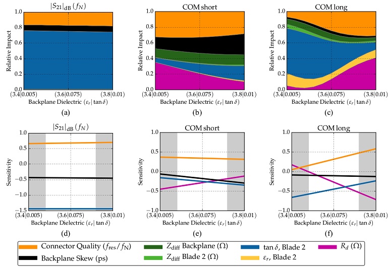
Figure 14: Relative impact of design parameters in the considered 100GBASE-KR4 link and most influential sensitivities by magnitude. The prediction is most accurate for the nominal case in the center of the depicted intervals. The outer skirts should be read with a grain of salt. The relative impact of parameters follows the intuition in case of , but is more involved in case of the COM ratio due to the relative measure of signal and noise quantities. The legend applies to all plots.

If changing the backplane material is not an option, for instance because of legacy support, the presented analysis reveals a couple of alternative factors worth considering. The FPM of the investigated link may be reduced by enforcing a higher quality of the connector and constraining the package termination impedance variation. In this, the dependencies of both COM short and COM long need to be considered jointly. Compliance requires that a link meets the specification in both cases.

Correlation of Parameter Sensitivity in COM and BER Analyses

COM unites loss, reflections, crosstalk, and device specifications to allow for a comparison of channels by means of a single figure of merit. On the other hand, the visual representation of received signal quality in the form of an eye diagram is an established and commonly used tool for BER analysis. The equivalence of COM and BER and the information they each convey are subject to ongoing discussion. However, a direct correlation between COM and BER was recently established in [9]. Therein, the equalized step responses generated from the COM algorithm are used as input to a full statistical simulation along with Tx and Rx noise.

In the experiments performed for this project, we used this flow as part of the framework in Figure 4 to generate eye diagrams directly from the COM algorithm. The opening is measured at a  according to Figure 15 for a correlation with the corresponding COM values.

COM and vertical eye opening V_EYE show similar trends with regard to relative impact and sensitivities of the design parameters as depicted in Figure 16. Note that the sensitivities are specific to the output quantities COM and V_EYE.

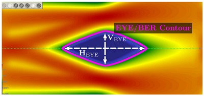
Figure 15: The eye opening is extracted as contour from eye plots at . The opening is characterized by means of the maximum vertical V_EYE and the maximum horizontal (H_EYE) opening.

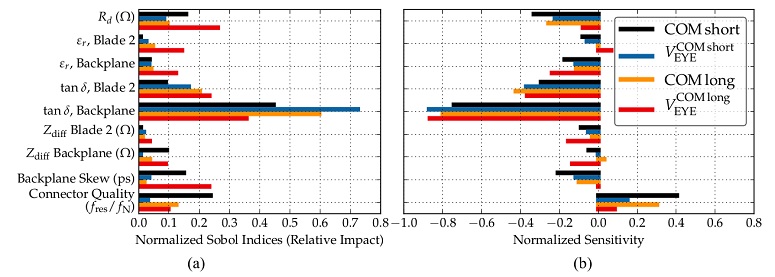
Figure 16: Correlating COM and equivalent vertical eye opening by means of (a) relative impact of input parameters and (b) corresponding sensitivities reveals a good correlation in capturing the trends. The horizontal eye opening shows little dependency with regard to the considered parameters. Values for COM correspond with Figure 12. The legend applies to both plots.

Hence, they are normalized for ease of comparison. The observed correlation suggests that eye diagrams can generally be considered equivalent to COM in screening parameter sensitivities and uncertainty.

Vice versa, COM reveals itself capable of capturing relevant trade-offs and parameter interactions. In a broader sense, this is encouraging for design flows and compliance checks that are based on eye diagram metrics. Figures of merit such as COM offer a simpler and computationally more efficient alternative to channel validation. This study confirms COM as a useful metric for parametric link design.

Conclusion

The proposed PCE work flow increases the efficiency and effectiveness of link design and validation. It extends compliance checks with additional information on the significance of design parameters and quantifies the consequences of their uncertainty. We provided code snippets that allow for prompt adaptation and uncertainty quantification for full-featured backplane links as well as subcomponents. Furthermore, the presented work flow integrates any preferred selection of tools and blends in with existing DoE flows. In fact, we highlight how the compatibility of methods enables thorough comparison and validation in this paper. In practice, the compatibility of PCE and RSM allows for a dual use of samples to cross-validate surrogate models at negligible cost. Moreover, segmented link analysis in particular benefits from ST, due to its structured sampling scheme.

The presented framework is general in its formulation and can be used for uncertainty quantification in mechanical PCB production in the same way at it was applied for a COM variability study. Additionally, the presented framework is well suited for educational use and yields insight into multifaceted relations between parameters as well as their joint impact on output quantities of interest. One general limitation governs all methods of uncertainty quantification and should be kept in mind: as the number N of stochastically independent variables increases, both PCE as well as RSM demand more samples to isolate and quantify each variable's impact. However, the proposed PCE/ST method is equally suited for computationally efficient stochastic screening as well as accurate analysis. Higher order polynomial orders P may be used in this.

This article has been previously published at DesignCon 2018 and received the Best Paper Award.

References

[1] P. Manfredi, D. V. Ginste, D. D. Zutter, and F. G. Canavero, “Generalized decoupled polynomial chaos for nonlinear circuits with many random parameters,” IEEE Microw. Wireless Compon. Lett., vol. 25, no. 8, pp. 505–507, Aug. 2015.

[2] J. B. Preibisch, T. Reuschel, K. Scharff, and C. Schuster, “Impact of continuous time linear equalizer variability on eye opening of high-speed links,” in IEEE Workshop Signal and Power Integrity (SPI), Turin, Italy, May 2016.

[3] J. B. Preibisch, T. Reuschel, K. Scharff, J. Balachandran, B. Sen, and C. Schuster, “Exploring efficient variability-aware analysis method for high-speed digital link design using PCE,” in DesignCon, Santa Clara, CA, USA, Jan. 2017.

[4] Y. Wang, S. Jin, S. Penugonda, J. Chen, and J. Fan, “Variability analysis of crosstalk among differential vias using polynomial-chaos and response surface methods,” IEEE Trans. Electromagn. Compat., vol. 59, no. 4, pp. 1368–1378, Aug. 2017.

[5] J. Feinberg and H. P. Langtangen, “Chaospy: An open source tool for designing methods of uncertainty quantification,” Journal of Computational Science, vol. 11, pp. 46–57, Aug. 2015.

[6] Z. Zhang, T. A. El-Moselhy, I. M. Elfadel, and L. Daniel, “Stochastic testing method for transistor-level uncertainty quantification based on generalized polynomial chaos,” IEEE Trans. Comput.-Aided Design Integr. Circuits Syst., vol. 32, no. 10, pp. 1533–1545, Oct. 2013.

[7] R. Mellitz, A. Ran, M. P. Li, and V. Ragavassamy, “Channel operating margin (COM): Evolution of channel specifications for 25 Gbps and beyond,” in DesignCon, Santa Clara, CA, USA, Jan. 2013.

[8] “IEEE Standard for Ethernet,” IEEE Std 802.3-2015 (Revision of IEEE Std 802.3-2012), Mar. 2016.

[9] V. Dmitriev-Zdorov, C. Filip, C. Ferry, and A. P. Neves, “BER- and COM-way of channel compliance evaluation: What are the sources of differences,” in DesignCon, Santa Clara, CA, USA, Jan. 2016.

[10] M. Dudek and N. Patel, “Package impedance and termination effect on COM,” in IEEE P802.3bs 200 GbE & 400 GbE Task Force Interim Meeting, New Orleans, LA, USA, May 2017. [Online]. Available: http://www.ieee802.org/3/bs/public/17_05/dudek_3bs_02_0517.pdf

[11] IEEE Computer Society, “IEEE standard for ethernet amendment 2: Physical layer specifications and management parameters for 100 Gb/s operation over backplanes and copper cables,” IEEE Std 802.3bj-2014 (Amendment to IEEE Std 802.3-2012 as amended by IEEE Std 802.3bk-2013), Sep. 2014.

[12] J. Antony, Design of Experiments for Engineers and Scientists, 2nd ed. Oxford, United Kingdom: Elsevier, 2014.

[13] R. H. Myers, D. C. Montgomery, and C. M. Anderson-Cook, Response Surface Methodology, 4th ed., ser. Wiley Series in Probability and Statistics. Hoboken, NJ, USA: John Wiley & Sons, Inc., 2016.

[14] K. Strunz and Q. Su, “Stochastic formulation of SPICE-type electronic circuit simulation with polynomial chaos,” ACM Trans. Model. Comput. Simul., vol. 18, no. 4, pp. 15:1–15:23, Sep. 2008.

[15] D. Xiu, Numerical methods for stochastic computations: a spectral method approach. Univ. Press, 2010. Princeton, NJ, USA: Princeton

[16] T. Crestaux, O. L. Maıtre, and J.-M. Martinez, “Polynomial chaos expansion for sensitivity analysis,” Reliability Engineering & System Safety, vol. 94, no. 7, pp. 1161–1172, 2009.

[17] B. Sudret and C. Mai, “Computing derivative-based global sensitivity measures using polynomial chaos expansions,” Reliability Engineering & System Safety, vol. 134, pp. 241–250, Feb. 2015.

[18] D. Xiu, “Fast numerical methods for stochastic computation: A review,” Communications in Computational Physics, vol. 5, no. 2-4, pp. 242–272, Feb. 2009.

[19] R. Rimolo-Donadio, X. Gu, Y. Kwark, M. Ritter, B. Archambeault, F. de Paulis, Y. Zhang, J. Fan, H.-D. Brüns, and C. Schuster, “Physics-based via and trace models for efficient link simulation on multilayer structures up to 40 GHz,” IEEE Trans. Microw. Theory Techn., vol. 57, no. 8, pp. 2072–2083, Aug. 2009.

[20] T. Reuschel, S. Müller, and C. Schuster, “Segmented physics-based modeling of multilayer printed circuit boards using stripline ports,” IEEE Trans. Electromagn. Compat., vol. 58, no. 1, pp. 197–206, Feb. 2016.

[21] P. Manfredi, I. Stievano, and F. Canavero, “Prediction of stochastic eye diagrams via IC equivalents and Lagrange polynomials,” in IEEE Workshop Signal and Power Integrity (SPI), Paris, France, May 2013.

[22] T. J. Robinson, Box-Behnken Designs. New Jersey, NJ, USA: John Wiley & Sons, 2014.

[23] H. Dsilva, S.-J. Moon, A. Zhang, C.-P. Kao, and B. Rothermel, “Mathematically de-mystifying skew impacts on 50G SERDES links,” in DesignCon, Santa Clara, CA, USA, Jan. 2017.