
This paper summarizes various methods for calibration of pulse generators, which are used for calibration of EMI receivers and spectrum analyzers with a quasipeak (QP) detector. Measurement receivers with a quasipeak (QP) detector are mainly discussed in European CISPR documents (CISPR – Comité International Spécial des Perturbations Rádioélectriques) and US standards ANSI 63.2 (QP parts derived from CISPR). In the last years, standards are being harmonized (international and national standards committees) and updated to reflect the current status of technology. The calibration of pulse generators is discussed in the standard EN 55016-1-1 [1], which is the harmonized version of the international standard IEC/CISPR 16-1-1 (currently Ed. 4 [2], yet this version has not been harmonized in European countries and it is likely the forthcoming Ed. 5 will be harmonized by 2020). (Annex B of [1] discusses the determination of pulse generator spectrum and Annex C discusses accurate measurements of the output of nanosecond pulse generators.) In the standard [1], only a very brief description of the methods is given, and technical details are hidden. The measurement uncertainty of the pulse generator characterization is not discussed.
The terminology in various standards (and also in different versions of the same standard) is sometimes not unique and confusing, however, all used quantities for characterization of pulse generators have dimensional units [V/Hz] or its mathematical equivalent. Different quantities used for QP detector calibration are listed in Table 1.
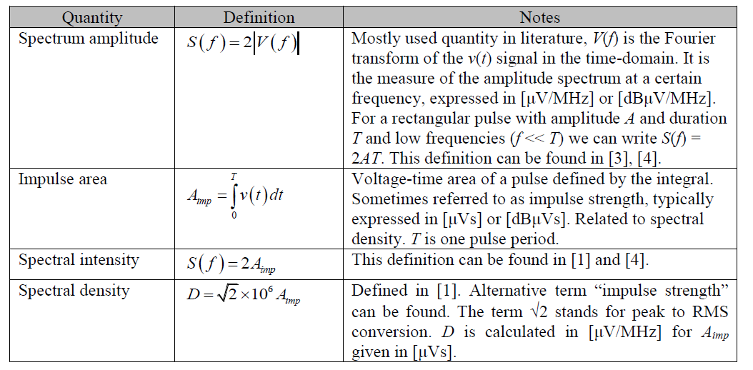
Table 1. Quantities used for characterization of pulse generators.
Pulse Generators
According to [1], a pulse generator is an instrument capable of generating time-domain rectangular pulses, or a pulse-modulated RF signal. Rectangular pulses are typically used for lower frequencies (bands A/B), pulse-modulated RF signals for higher frequencies (bands C/D) because of the risk of receiver damage due to high peak voltages, see Tab. 2. In order to limit intermodulation effects in measuring receivers, the spectrum above the upper limit of the frequency band shall be limited [1] (10 dB down at twice the upper frequency). The base-band pulse generators is usually comprised of an energy-storage device (electrostatic, magnetic field) and a switch which discharges a fraction or all of the energy into a load.
In the past, the switch was realized using a mechanical mercury relay, in current designs, the mercury relay is replaced by other mechanical principles or a solid-state semiconductor switch is used. Very often the storage device is a charged coaxial line, whereas the pulse duration is given by the electrical length of the line and the impulse area is given by the charge voltage. The charged transmission line does not allow for very fast rising edges, and thus other principles are currently used, such as a nonlinear transmission line, step-recovery diode or avalanche transistors. Example of rectangular pulse parameters is given in Tab. 2 and a spectrum of a rectangular pulse is shown in Fig. 1.
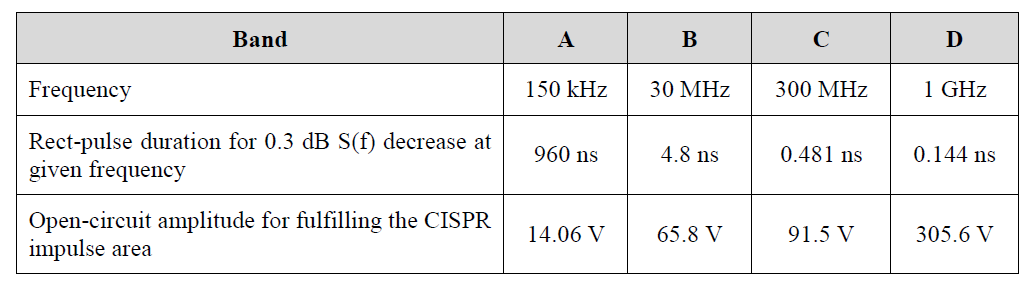
Table 2. Example of rectangular pulse parameters.

Figure 1. Typical spectrum of a rectangular pulse.
The pulse-modulated RF generator uses a harmonic signal with a pulse envelope. The spectrum is similar to a rectangular pulse (upconverted to the carrier frequency fc), maximum of the spectrum is at fc. The spectrum is uniform in a given bandwidth, which implies that pulses with longer duration can be used with lower amplitudes compared to baseband pulse generators (lower risk of measuring receiver damage). The time-domain signal and its spectrum are schematically shown in Figure 2.
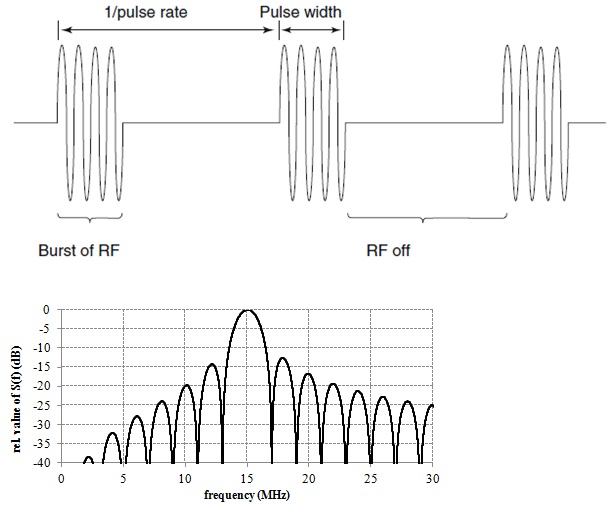
Figure 2. Pulse-modulated RF pulse in the time domain (left) and in the frequency domain (right).
The spectrum amplitude is calculated as follows
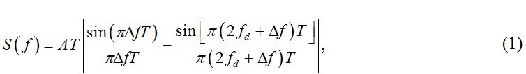
where 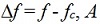 is the peak pulse amplitude and T is the pulse duration. Generally, the spectrum is not perfectly symmetrical around the carrier frequency (see Figure 2 right), however, in a narrow band around the carrier frequency and for >15 periods of the RF carrier in the pulse, the spectral non-symmetry is negligible. The spectrum amplitude at the carrier frequency is calculable from the RF power and pulse duration. An example of RF pulse parameters is given in Table 3.
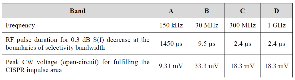
Table 3. Example of RF pulse parameters
Calibration methods in this paper are demonstrated on the calibration of the CISPR pulse generator Schwarzbeck IGUU2916, ser. no. IGUU2916164 (base-band pulse generator, characterized within the project interlaboratory comparison, activity A3.1.2). The generator is shown in Figure 3. The methods are compared, and the best method with regards the measurement uncertainty, feasibility, and required instrumentation is chosen.
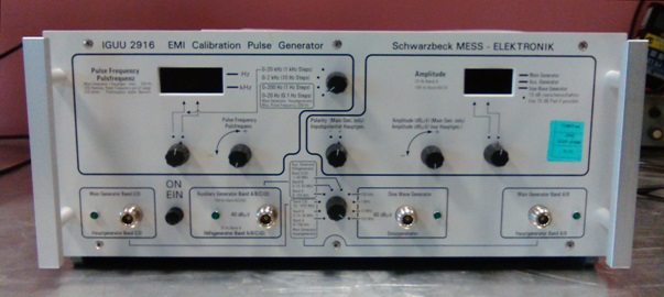
Figure 3. CISPR pulse generator Schwarzbeck IGUU 2916.
Calibration Methods
A pulse generator can be characterized using several methods. For the purpose of this paper, the Main generator Band A/B or Main generator Band C/D output of the IGUU2916 generator was used (see sections 3.1, 3.2 and 3.3) and the Auxiliary Generator Band A/B/C/D was used (see section 3.4). The polarity was always (+), and the amplitude of the main generator was always 60 dBμV. The amplitude of the auxiliary generator was 40 dBμV (maximum available amplitude). The pulse repetition rate was changed according to the band. In the EN 55016-1-1 (CISPR 16-1-1) there are specified impulse areas of a typical generator for both open-circuit and 50 Ω load, see Table 4. The values in this paper correspond to the measurement of the spectrum amplitude (calculated from the impulse area) into 50 Ω nominal load.
Table 4. Impulse area of a generator for different bands specified in the EN 55016-1-1 standard.
Fourier transform of time-domain pulse waveform
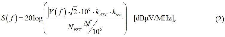
The spectrum amplitude is determined by direct acquisition of the pulse generator output voltage using an oscilloscope and conversion to the frequency domain. For this purpose, a digital real-time oscilloscope (DRTO) or an equivalent-time sampling oscilloscope (DSO) can be used. The method is useful for baseband pulse generators; it is simple and time efficient. Corrections for the cable (attenuator) properties and oscilloscope transfer function must be performed. A DRTO triggers directly the measured pulse. The traceability of DRTO is complicated due to the nonlinear behaviour of modern analog to digital converters and the transfer function correction. A DSO needs an external trigger signal, which is usually derived from the measured signal itself (approx. 20 ns delay line is used). The measurement is traceable to the electro-optic sampling system. A general diagram of the measurement setup using the DRTO and DSO is shown in Figure 4. Typically, 20 to 50 acquisitions of each pulse are taken in order to calculate the type A uncertainty.
Figure 4. Typical measurement setup with use of a DRTO (left) and DSO (right).
The measurement equation is the following:
where V(f) is a Fourier transform of the voltage trace from oscilloscope in [V], NFFT is the FFT length, Df is the frequency resolution in [Hz], kATT is the total attenuation of the signal path, that is, the cables and external attenuators connected between the generator and oscilloscope, (1), kosc is a factor taking into account the oscilloscope frequency response (1).
A cable with attenuators on both sides should be used in order to reduce the pulse amplitude and improve the mismatch uncertainty. The attenuation of the cable + attenuators and the reflection coefficient is measured using a vector network analyzer, and the calculated frequency-dependent spectrum amplitude is then corrected for the measured attenuation at each frequency. The oscilloscope transfer function is taken into account by adding a small contribution to the measurement uncertainty. A full deconvolution of the oscilloscope transfer function from the measured voltage trace is difficult to perform, as the phase response of the oscilloscope is not easily measurable (modern high-speed DRTOs cannot be regarded as linear time-invariant systems).
The following text shows an example of measured and calculated results and the associated measurement uncertainty. Further details about the concept of the measurement uncertainty can be found in [5]. The statement of the result of a measurement is complete only if it contains both the measured value and the uncertainty of measurement. The measurement uncertainty characterizes a dispersion of the values that could be reasonably attributed to the measured value with certain probability distribution. In metrology, a coverage factor k = 2 is used to express that the measured value coverage interval is 95 % for Gaussian-like probability distribution of the measured quantity. The spectrum amplitude was calculated using (2) from oscilloscope voltage samples corrected for the cable and attenuator and oscilloscope transfer function. The following measurement uncertainty contributions apply:
- impedance mismatch correction between device 1 and 2 (e.g. between a generator and cable)
 (dB), where G1 and G2 are linear reflection coefficients of devices 1 and 2, respectively,
 - type A uncertainty was calculated from repeated calculations of the spectrum amplitude for all captured time traces, its value was determined from n measurements in a standard way as
 .
.
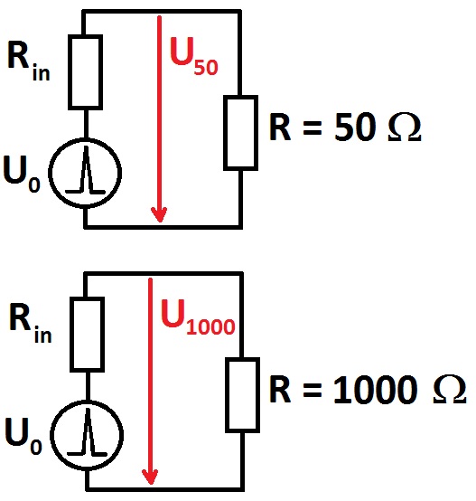
Figure 5. Measurement of the pulse generator output reflection coefficient.
The inner resistance of the generator is calculated as follows
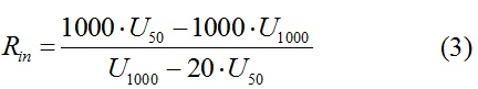
and the output reflection coefficient (magnitude only) is then
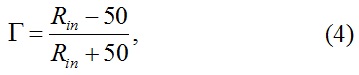
whereas the system characteristic impedance 50 Ω is assumed. The uncertainty of the reflection coefficient is dependent on the accuracy of the oscilloscope voltage measurement and attenuation of the voltage divider (1000 Ω) or cable + attenuator (50 Ω). Typical pulse shapes for different CISPR bands into 50 Ω load are shown in Figure 11, typical pulse shapes for different CISPR bands into 1000 Ω load impedance are shown in Figure 6.
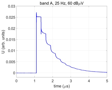
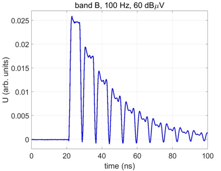
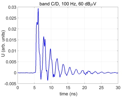
Figure 6. Pulse shape into 1000 Ω load impedance, bands A/B/C/D, voltage in arbitrary units.
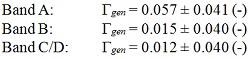
The calculated generator output reflection coefficient is as follows:
The measured results of the Fourier transform method are summarized in Table 5 together with the equivalent QP level which is compared to the actual amplitude setting. The equivalent QP level is calculated as
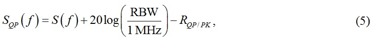
where RBW is the actual filter resolution bandwidth (200 Hz for band A, 9 kHz for band B and 120 kHz for bands C/D) and RQP/PK is the ratio of the peak/quasi-peak (dB) for the pulse repetition rate specified for each band (see Table 7 in [1]).
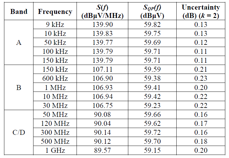
Table 5. Measured results of the Fourier transform method; IGUU 2916 Main generator, amplitude setting 60 dBμV.
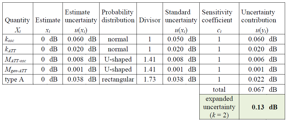
Table 6. Example of uncertainty calculation, band A, frep = 25 Hz, frequency 9 kHz.
Intermediate-frequency (IF) measurement method
This method uses an EMI measuring receiver and its IF output. It is referred to as a “video pulse technique” in MIL-STD-462 [7], and it is referred to as “video pulse technique” and “area method” in [1]. The method uses a pulse signal and a reference CW signal (with known level) connected to a narrow-band filter, whereas the output of the filter (IF) is acquired using an oscilloscope. The spectrum amplitude is then calculated from the response to both input signals at the frequency of the tuned filter (receiver) as follows

where Urms (V) is the level of CW signal which causes equal oscilloscope reading as the pulse signal, IBW (Hz) is the impulse bandwidth of the used filter. The accuracy of the method is dependent on the accurate characterization of the receiver impulse bandwidth IBW. The spectrum amplitude is calculated as the surface under the pulse envelope (i.e. positive amplitudes only), see Figure 7. The measurement setup is shown in Figure 8.
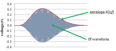
Figure 7. IF measurement method.
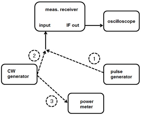
Figure 8. Measurement setup of the IF method.
The practical procedure is: first, the pulse signal from the generator is input to the receiver and the response of the receiver’s filter is captured using an oscilloscope (direct connection using a high-grade cable, without attenuators). The peak-to-peak amplitude of the trace is measured as well. In the second step, a CW sine signal is input to the receiver, and its amplitude is changed until the oscilloscope peak-to-peak reading is the same as for the pulse signal. The RMS level of this sine signal is measured using a calibrated power meter (or voltmeter at low frequencies). The attenuation of the cable from the generator to the receiver and from the receiver IF output to the oscilloscope is not important, as it cancels due to the ratio measurement. The measurement equation is following
where Vpwm,rms is the voltage across a 50 Ω load of the CW sine signal calculated from the RMS power measured by the power meter in [μV]
Venv is the amplitude of the IF pulse envelope (see Fig. 9) in [V]
Vosc,pp is the peak-to-peak amplitude of the receiver response (IF output) to a CW sine signal measured by the oscilloscope in [V]
IBW is the receiver impulse bandwidth in [Hz]
kpeak takes into account the uncertainty of the peak ratio of the response to pulse/CW signal (dimensionless)
kosc takes into account the oscilloscope frequency response (dimensionless)
kIBW takes into account the uncertainty of the determination of the impulse bandwidth (dimensionless).
The receiver impulse bandwidth is calculated as
where Venv is the amplitude of the IF pulse envelope (see Fig. 9) in [V]
X is the oscilloscope horizontal resolution in [s/div]
N is the number of samples of the envelope [-]
venv,k represents the k-th sample of the IF pulse envelope in [V]
10 takes into account the number of oscilloscope horizontal screen divisions.
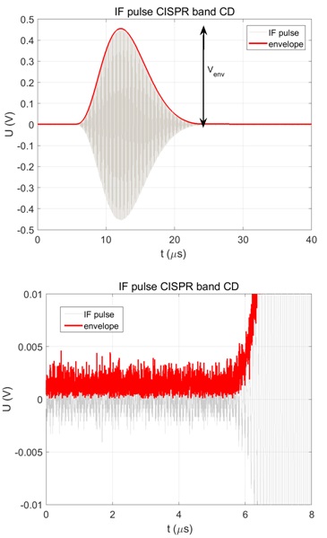
Figure 9. Response of the receiver to a pulse signal + envelope of the signal (left), unfiltered envelope (right).
The determination of the IF pulse envelope can be done using different methods, which results in slightly different calculated receiver impulse bandwidth and consequently spectrum amplitude. Either the envelope can be calculated as a moving average of the voltage IF trace (with e.g. 50 - 200 samples window), or it can be calculated as a magnitude of the Hilbert transform of the IF voltage trace (time domain). It is convenient to filter the envelope trace using a low-pass filter in order to remove the noise (which is obvious in Figure 9 right). The area under the envelope is then calculated as a sum of the voltage samples divided by the number of envelope samples.
The spectrum amplitude was calculated using (6) from oscilloscope samples of the voltage at the IF output of an EMI receiver. Both the receiver’s response to pulses and to an equivalent sine CW signal was acquired. The oscilloscope traces are well repeatable (small type A uncertainty), however the determination of the impulse bandwidth from the IF pulse envelope may not be a unique task. The IF pulse envelope was calculated as a magnitude of the Hilbert transform of oscilloscope samples

where venv is the discrete envelope of the oscilloscope samples vosc, symbol H(.) denotes the Hilbert transform and operator (*) stands for convolution in the time domain.
The Hilbert transform was implemented in MATLAB using command hilbert(x). Removing noise at the beginning and the end of the calculated envelope influences the calculated impulse bandwidth and consequently the spectrum amplitude. This process is taken into account as a part of the total uncertainty of the spectrum amplitude.
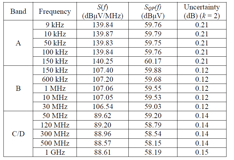
Table 7. Example of measured results, IGUU 2916 Main generator, amplitude setting 60 dBμV.
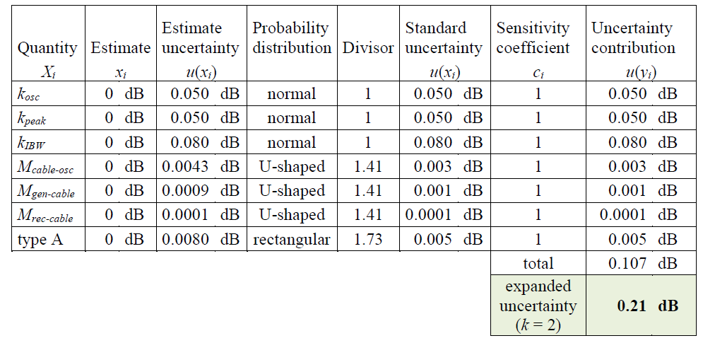
Table 8. Example of uncertainty calculation, band A, frep = 25 Hz, frequency 9 kHz.