Like any good tradesman, every electronic design engineer should carry a variety of tools in their toolbox. Some of the tools I like to carry are transmission line equations. At this point you might ask yourself the question, “Why use equations, when I can just use a 2D or 3D field solver to give me the answer and a whole lot more?” One answer is practical intuition. Sometimes it is useful to have a way to check the accuracy of a field solver for which there are exact equations. Or, as my friend Eric Bogatin likes to say, “Sometimes an answer now is better than a good answer late.” 

In almost all cases, equations are approximations. However, there are three unique cross-sectional geometries that have exact equations. They are twin-rod, rod-over-plane and coaxial. All three assume the dielectric material is homogeneous and completely fills the space when there are electric fields.

The first transmission line is the twin-rod geometry. An example of this is 300 Ohm twin-lead flat cable. It was once used almost exclusively for RF transmission between antenna and TV sets. But, with the popularity of cable and satellite TV over the years, it has given way to coaxial cable due to its superior noise rejection and shielding effectiveness.

Figure 1illustrates the electromagnetic field relationship of a twin-rod geometry when driven differentially. As current propagates along one rod, an equal and opposite current flows along the other one.

Shown on the left is the electric field with a capacitance (C) between the two rods, and twice the capacitance (2C) from each rod to a virtual return plane. It is called that because if a real conducting plane was placed in the same position, the electromagnetic fields would look exactly the same between the two rods; thus resembling the second transmission line, rod-over-plane, described later.

The right half of the figure shows the magnetic-field loops and direction of rotation around each rod. There is only one loop shown for clarity. But in reality, the number of loops is a function of the amount of current and the length of the rods. The counter-rotating loops of current forms a virtual return at exactly one half of the space between the two rods.

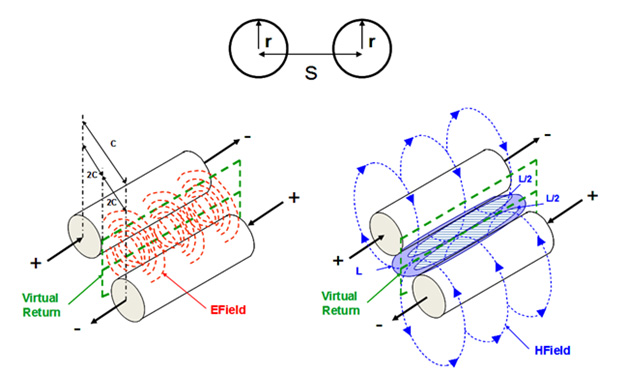
Figure 1. Twin-rod geometry showing electromagnetic field relationship. E-field is shown in red (left) while H-field is shown in blue (right).

In his book, “Signal Integrity Simplified”, Eric Bogatin defines the loop inductance as, “the total number of field line loops around a conductor per amp of current” and the loop self-inductance as, “the total number of field line loops around a conductor per amp of current in the same loop”. Applying these definitions to the figure, the loop inductance (L) is the inductance between the two rods, and the loop self-inductance (L/2) is the loop self inductance to the virtual return plane, which is equal to one half the loop inductance.

Thus, the relationships between capacitance, inductance and impedance of a twin-rod geometry are described by the following equations:

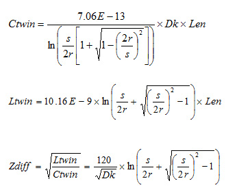
Where:

Ctwin= Capacitance between twin-rods - F

Ltwin= Loop Inductance between twin-rods – H

Zdiff = Differential impedance of twin-rods - Ω

Dk= Dielectric constant of material

Len= Length of the rods - inches

r= Radius of the rods - inches

s= Space between the rods - inches

Because the electro-magnetic fields create a virtual return plane at exactly one half of the spacing between the rods, each rod behaves like a single rod-over-plane geometry as illustrated in Figure 2.

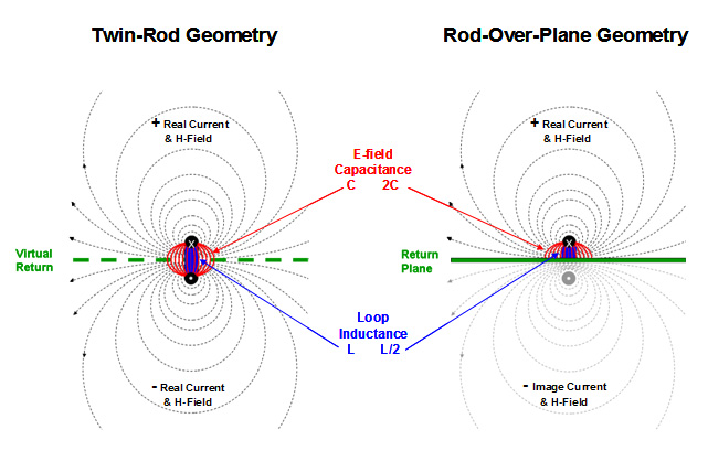
Figure 2. Electromagnetic fields comparison of twin-rod (left) vs. rod-over-plane (right) geometries.

Whenever an AC current carrying conductor is in close proximity to a conducting plane, some of the magnetic-field lines penetrate it.  When the current changes direction, the associated magnetic-field lines also change direction, thereby causing small voltages to be induced in the plane. These voltages create eddy currents, which in turn produce their own magnetic-fields.

Eddy current-induced magnetic-field line patterns look exactly like magnetic-field lines from an imaginary current below the plane; located the same distance as the real current above the plane. This imaginary current is called an image current and has the same magnitude as the real current; except in the opposite direction. The image current creates associated image magnetic-field lines in the opposite direction of the real field lines. As a result, the real magnetic-field lines are compressed between the rod and the plane. Since the rod-over-plane geometry has only one rod, the loop inductance is the same as the loop self-inductance.

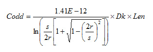
For a twin-rod geometry, the odd mode capacitance, Codd, is the capacitance of each rod to virtual return plane. It is equal to twice the capacitance between rods, and is equivalent to the rod-over-plane capacitance. 

Likewise, the odd mode inductance, Lodd, is the inductance of each rod to the virtual return plane.  It is the same as the loop inductance of rod-over-plane and thus equal to one half the inductance between rods.

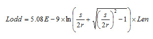
The odd mode impedance of each rod is half of the differential impedance, and is equivalent to the rod-over-plane impedance.

Last, but not least, the third transmission line is the coaxial (coax) geometry, as described by Figure 3. It consists of a center conductor; imbedded within a dielectric material; surrounded by a continuous outer conductor; also known as the shield. Both share the same geometric center axis; hence the name coaxial. It is common practice to transmit the signal on the center conductor, while the outer conductor provides the return path for current back to the source. The shield is usually grounded at both ends.

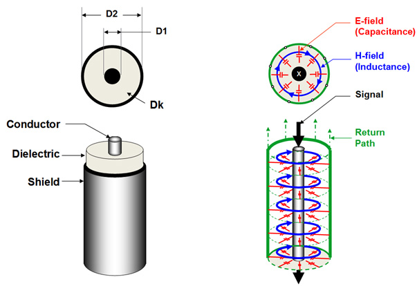
Figure 3. Example of a coaxial transmission line geometry and the electromagnetic field patterns with respect to the current through the structure.

As the signal propagates along the transmission line, an electromagnetic field is set up between the outer surface of the center conductor and the inner surface of the shield. As illustrated in red, the electric E-field pattern sets the capacitance per unit length, and the magnetic H-field, in blue, sets the inductance. For the center conductor, the “X” represents current flowing into the page and the “.” (dots) within the shield ring is current flowing out of the page.

Figure 4 describes the magnetic-field relationship for a coaxial geometry. As current propagates along the center conductor, concentric magnetic-field lines (blue) are created in the direction as shown following the right hand rule.

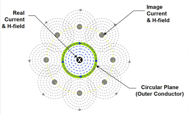
Figure 4. Magnetic-field relationship of a coaxial transmission line geometry showing associated real and image currents.

Like the rod-over-plane geometry, whenever an AC current carrying conductor is in close proximity to a conducting plane, some of the magnetic-field lines penetrate it. Now imagine taking that conducting plane and wrapping it entirely around a center conductor to form the coaxial structure. Some of the magnetic-field lines then penetrate the entire circumference.  When the AC current changes direction, the associated magnetic-field lines also change direction, causing small voltages to be induced in the outer conductor. And, like the rod-over-plane geometry, these voltages create eddy currents, which in turn, produce their own magnetic-fields.

Eddy current-induced magnetic-field line patterns look exactly like magnetic-field lines (grey) from imaginary currents surrounding the outer conductor. These imaginary currents are referred to as image currents, and have the same magnitude as the real current, except they are in the opposite direction. For simplicity, there are only eight image currents shown. But in reality, there are many more; forming a continuous loop of imaginary currents on a radius equal to twice the radius of the outer conductor to the center of the circle. The image currents create associated image magnetic-field lines in the opposite direction of the real field lines. As a result, the real magnetic-field lines (blue) are compressed and are entirely contained within the outer conductor.

The outer conductor thus forms a shield preventing external magnetic-fields from coupling noise onto the main signal and likewise, prevents its own magnetic field from escaping and coupling to other cables or equipment. This is why it is a popular choice for modern RF applications.

The relationships between capacitance, inductance and impedance of a coaxial structure can be expressed by the following equations:

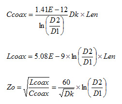
Where:

Ccoax= Capacitance - F

Lcoax = Inductance – H

Zo = Characteristic Impedance – Ohms

Dk= Effective Dielectric constant

Len= Length of the rods

D1= Diameter of conductor

D2= Diameter of shield

References:

[1] E. Bogatin, “Signal Integrity Simplified”. Englewood Cliffs, NJ: Prentice-Hall, 2004.

[2] H. Johnson, M. Graham,”High-Speed Signal Propagation”. Upper Saddle River, NJ: Prentice-Hall, 2003.

Bert Simonovich was born in Hamiton, ON, Canada. He received his Electronic Engineering Technology diploma from Mohawk College of Applied Arts and Technology, Hamilton, ON, Canada in 1976. Over a 32-year career, working as an Electronic Engineering Technologist at Bell Northern Research and later Nortel, in Ottawa, Canada, he helped pioneer several advanced technology solutions into products. He has held a variety of engineering, research and development positions, eventually specializing in signal integrity and backplane architecture for the last 10 years. He is the founder of Lamsim Enterprises Inc., where he continues to provide innovative signal integrity and backplane solutions to clients as a consultant.