Editor's Note: This is the second of a two-part series on antenna anechoic chamber design. Part one, published in the January 2016 issue, discussed absorber requirements for rectangular, far field ranges. Part two discusses compact ranges and near field measurements.
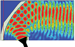
Figure 1 Simulated results of a parabolic reflector, showing plane wave behavior on the right.
The task of adequately specifying performance for an indoor anechoic chamber without driving unnecessary costs or specifying contradictory requirements calls for insight that is not always available to the author of the specification. Although there are some articles and books1-3 that address anechoic chamber design, a concise compendium of reference information and rules of thumb on the subject would be useful. This second part of the series intends to do that, concentrating on the sizing of compact ranges and chambers for near field systems. As was done in part one, simple approximations are used for absorber performance to generate a series of equations that help specify performance and size of facilities.
Part one of this series identified limitations in using far field chambers, mainly related to the electrical size of antennas that can be tested. As was shown, an 18" dish used by a popular satellite TV service will be almost impossible to test in a far field chamber. The satellite service operates at 18.55 GHz, the dish antenna is 28.29 wavelengths (λ) in size, so the far field is at approximately 1600 λ or 25.9 m (84.8 ft). Clearly for such an electrically large antenna, far field illumination indoors is not economically feasible. For this antenna, a compact range or near field measurement is more suitable.
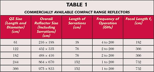

Figure 2 A typical compact range layout showing the reflector pattern, side (a) and top (b) views. At 2 GHz, the energy incident on the side walls, floor and ceiling is more than 40 dB down.
COMPACT RANGES
Although barely mentioned in the IEEE standard test procedure for antennas,4 the compact range (CR) has become an important tool for measuring electrically large antennas. The CR uses a parabolic reflector to create a plane wave illumination at the location of the antenna under test (AUT). This plane wave simulates the field distribution that the antenna experiences in the far field. Figure 1 shows a parabolic reflector illuminated by a source located at the focal point of the parabola. The plane wave behavior can be seen a short distance from the reflector. The reflector system is the controlling factor when sizing the range. The reflector must be large enough to provide a plane wave that illuminates the entire antenna being tested, and the reflector should be properly terminated. The purpose of the termination is to reduce the effects of the terminated paraboloid on the illumination. The two most common ways of terminating a reflector are serrations and rolled edges.6 In the case of serrated edge reflectors, serrations can be between 3 λ and 5 λ at the lowest frequency of operation. Table 1 provides a typical list of reflectors, showing their overall size and frequency ranges. Note that as frequency increases, the reflector becomes more efficient. While some reflectors can operate well into the millimeter wave range, extra care should be taken during manufacturing and surface finishing, as surface imperfections will affect the performance.
Reflector size is the determining factor when sizing the width and height of the chamber. The length of the chamber will be affected by the focal length of the reflector. The distance from the vertex of the reflector to the quiet zone (QZ) is given by the following rule:

where fl is the focal length of the reflector. Referring to the satellite TV antenna, requiring a far field distance of 25 m to test, one might expect long chambers and large distances for CR testing. However, Table 1 with Equation 1 indicates the test distance for a 61 cm QZ is 3 m. This is sufficient to test the satellite TV antenna.
As a rule, the length of a CR chamber is given by the following equation:

where Rclr is the reflector clearance. This includes the mechanical structure to support the reflector, which ranges from 60 cm to 2 m, depending on the overall reflector size. In general, the wall behind the reflector has a small absorber, usually λ/2 in thickness, and only covers the perimeter of the wall. The parameter t is the thickness of the end wall absorber. For a CR, this is the most critical wall and should have the lowest reflectivity; it is recommended the value of t be no less than 3 to 4.
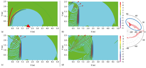
Figure 3 Wave propagation from the source horn vs. time – 6.6 ns (a) 10.4 ns (b) 11.3 ns (c) 15.1 ns (d) – compared to the far field pattern.
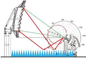
Figure 4 Absorber on the floor between the feed positioner and the reflector is critical to reduce the reflected energy from illuminating the reflector.
The width of the chamber is calculated using:

where CRw is the overall width of the reflector. There is an additional 2 λ from the tips of the serrations to the absorber tips on each side of the reflector, although in some cases the spacing can be as small as one wavelength on each side. The final item determining the width of the range is the thickness of the absorber.
While for far field ranges the absorber on the ceiling, floor and side walls should be thick enough to provide good bistatic reflectivity at oblique angles, in the CR the side wall absorber does not need to be as thick. Figure 2 shows a typical CR chamber. The radiation pattern of the CR reflector has been superimposed over the chamber drawing. The reflector in the figure provides a 3.66 m × 1.82 m elliptical QZ. The depth of the QZ is 3.66 m. The important aspect of the CR is that it has a very directive pattern, with directivities in excess of 25 dBi. As Figure 2 shows, the energy incident on the absorber on the side walls is already 40 dB below the direct path. A 1 λ thick absorber will provide 10 dB of absorption at over 60 degrees of incidence (see Figure 4 in part one, published in January 2016). Combining the reflectivity with the difference in magnitude between the direct ray and the reflected ray, results in a reflected energy level of approximately -50 dB. The reflector is being used in the near field while the radiation pattern of the reflector is a far field concept. However, this is an acceptable approximation, as it provides a method for estimating the level of energy that radiates from the reflector in the direction of the walls. As Figure 3 shows, the reflector will send some energy towards the side walls, estimated from the far field pattern of the reflector.
The height of the chamber has a similar equation for calculating the size:

where CRh is the overall height of the reflector. The spacing between the tips of the reflector and the tips of the ceiling absorber is 2 λ. The parameter K provides a factor for the spacing between the floor and the reflector. For the floor absorber, we want a larger separation between the edge of the reflector and the tips of the floor absorber. This reduces the angle of incidence at the specular point between the reflector feed and the reflector to minimize the impact of the floor reflection on the reflector illumination (see Figure 4). Equation 4 includes K wavelengths of space between the tips of the floor absorber and the serration tips. K should be large enough to provide sufficient space for the feed positioner supporting the feed antenna that illuminates the reflector. As was the case with the side walls, the absorber on the floor and the ceiling can be 1 λ thick. Special consideration must be given to the floor absorber between the feed and the reflector, which may be 2 λ thick. In general, the absorber electrical thickness at the lowest frequency can be t ≤ 1.2 and t ≥ 0.75 for the side wall and ceiling treatments, respectively.
NEAR FIELD RANGES
Different techniques are used for performing near field measurements; they align with the type of antenna being measured. With all approaches, the field (amplitude and phase) radiated from the AUT is measured on a surface, and the far field behavior is derived mathematically from this measurement. Three different near field techniques — planar (PNF), cylindrical (CNF) and spherical (SNF) — represent the surface where the data is measured.7-9 The most basic near field measurement approach is planar scanning, where the field radiated from the antenna is scanned on a single plane. This is a good technique for high gain antennas, as there is a very small amount of energy radiating to the back of the antenna. Cylindrical scanning is where the field is measured on the surface of a cylinder excluding the top and bottom surfaces. This is ideal for long antennas that are omnidirectional or have a wide beam on one of the principal planes but a narrow beam in the perpendicular plane. Spherical scanning is a more general measurement approach. Here the field is measured on a sphere that contains the entire antenna. In general, the test distance for PNF measurements is between 3λ and 10λ. For SNF, the probe can be further away.
The same equations developed for far field chambers can be used for SNF with the exception of the test distance. In general, the equation is given by:

where dpp is the depth of the probe (measuring antenna) and its positioner. The variable n is the diameter in wavelengths of the minimum sphere that contains the AUT. The absorber on the two end walls will have a thickness of teλ, where te is the thickness, in wavelengths, of the end wall absorber. As is customary, 2λ is added between the minimum sphere and the absorber tips. Finally, 4λ is estimated to be the distance between the probe and the sphere containing the antenna.
The width of the SNF chamber is given by:

In this case, ts is the thickness, in wavelengths, of the side wall absorber. This is a rough approximation. For both Equations 5 and 6, a minimum of 1 meter should be added to prevent the positioning equipment from hitting the probe as it rotates the antenna being measured. The chamber also should provide room for people to work inside to set up the measurement. This is more critical for higher frequencies (above 2 GHz), where the 4λ separation may not be enough for the positioner to clear the probe.
The angle of incidence onto the side absorber is:

Taking the limit as n → ∞, θ < 63.4 degrees. Using the absorber approximations presented in part one of this series, we can estimate that ts ≈ 2te. To do this, we check the reflectivity of the end wall absorber at normal incidence and select the thickness of the absorber that will provide similar reflectivity for the 63.4 degree incident angle. The ceiling and the floor will have the same absorber as the side walls.
The chamber height can be estimated using the following equation:

where the variable hp accounts for the height of the positioning equipment. In a typical roll-over azimuth positioner used in SNF measurements, hp should include the height of the floor slide, the azimuth positioner and the offset slide. The positioning equipment in the far field chamber equations or the CR equations (except for the feed positioning) is not an issue because other dimensions are so dominant in these ranges (i.e., the far field test distance or the reflector size).
PNF systems use a planar scanner to measure highly directive antennas (i.e., gain > 20 dB). The high gain of the AUT benefits the design of the range, as some regions of the range do not need to be treated with absorber, such as those behind the AUT. The test distance, as stated above, is between 3λ and 10λ. The dominant factor for sizing a PNF range is the scanner, where the scan size is given by:

θs is the maximum angle for accurate far field and nλ is the electrical size of the antenna being tested (see Figure 5). The variable k is the test distance in wavelengths; hence, 3 < k < 10. The physical scanner will usually be slightly larger than the scan plane. Typically, 2λ is the separation to the absorber tips.

Figure 5 Geometry of a planar near field measurement.
The width of the range becomes:

where Δscn is the additional space required for the scanner structure, and ts is the thickness of the absorber.
The length of the range is given by the following equation:

Where Sclr is the scanner depth, which should include the spacing to the absorber, if any (the scanner can be placed very close to the tips), and the probe length. Ad is the depth of the AUT and the support structure for aligning that antenna with the scanner. The 4λ in Equation 12 is the space between the back of the AUT and the range wall. For very high gain antennas, this wall does not need absorber treatment. If absorber is desired, the thickness of absorber for this wall can be as small as λ/4. The thickness of the absorber on the wall behind the scanner takes advantage of the directivity of the probe used to scan the plane. Thus, t ≥ 2.
The remaining value to be defined is the absorber on the side walls. This is dependent on the angle θs and the factor k. The width is approximated as:

Using the approximation that

Notice that the angle of incidence is only dependent on the size of the AUT, the maximum angle for accurate far field and the test distance in wavelengths. Figure 6 shows that even at 10λ for a test distance, the largest angle of incidence is close to 20 degrees. From the absorber approximations presented in part one, the reflectivity of a given piece of absorber of certain electrical thickness does not deteriorate much within that range of angles of incidence. If the AUT is a simple passive antenna, the high gain can be a benefit. Since the antenna will not radiate much energy to the side walls, a smaller absorber (t < 1) may be used. However, if the AUT is a complex antenna with beam steering, then the side walls should have more thickness (t ≥ 2).
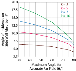
Figure 6 Angle of incidence on the side wall absorber vs. maximum angle for accurate far field patterns, plotted for several test distances. The antenna aperture is 20λ.
The height of the chamber should be calculated in the same way as the width. In some cases, the scan distance is different between vertical and horizontal; it is not rare for the chamber to have a non-square cross section. The equation for the height is:

Where yo is the minimum height of the probe, i.e., the location of the probe at the bottom of the vertical motion. This includes the rails on which the scanner moves in the horizontal axis and should also be large enough to include the floor absorber; at a minimum, yo > tsλ.
The above rules for SNF and PNF ranges can be combined to arrive at a range size for a CNF system.
CONCLUSION
Part two of this series provided an overview of the rules and physics that guide the selection and sizing of indoor anechoic chambers for compact ranges and for near field scanning measurements. All the equations are approximations. The length, in most cases, is a minimum; more space may be required for the loading and unloading of the AUT, changing feeds and range antennas and connecting additional equipment. Both parts of this series provide a general overview and equations for sizing anechoic rooms for the most common antenna measurement methods currently being used.
References
- L. Hemming, “Electromagnetic Anechoic Chambers: A Fundamental Design and Specification Guide,” IEEE Press/Wiley Interscience: Piscataway, N.J., 2002.
- G. Sanchez and P. Connor, “How Much is a dB Worth?,” 23rd Annual Symposium of the Antenna Measurement Techniques Association (AMTA), Denver, Colo., October 2001.
- J. Hansen and V. Rodriguez,“Evaluate Antenna Measurement Methods,” Microwaves and RF, October 2010, pp. 62267.
- ANSI/IEEE STD 149-1979 149-1979 - IEEE Standard Test Procedures for Antennas, 1979, reaffirmed 2008.
- J.R.J. Gau, D. Burnside and M. Gilreath “Chebyshev Multilevel Absorber Design Concept,” IEEE Transactions On Antennas Propagat., Vol. 45, No. 8, pp. 128621293, 1997.
- T.H. Lee and W. Burnside, “Performance Trade-Off Between Serrated Edge and Blended Rolled Edge Compact Range Reflectors,” IEEE Transactions on Antennas and Propagation, Vol. 44, No. 1, January 1996, pp. 87296.
- D. Hess, “Near-Field Measurement Experience at Scientific Atlanta,” White Paper, www.mitechnologies.com/papers/91/Near-Field%20Measurement%20Experience%20at%20Scientific-Atlanta.pdfhttp://www.mitechnologies.com/papers/91/Near-Field%20Measurement%20Experience%20at%20Scientific-Atlanta.pdf.
- Yaghjian, “An Overview of Near-Field Antenna Measurements,” IEEE Transactions on Antennas and Propagation, Vol. AP-34, No. 1, January 1986, pp. 30245.
- J. E. Hansen ed., “Spherical Near-Field Antenna Measurements,” IEEE Peter Peregrinus Ltd.: London, UK, 1988.
Vince Rodriguez is a senior applications engineer with MI Technologies in Suwanee, Ga., where he brings his expertise in numerical modeling, RF absorber and anechoic range design to the design of antenna, radar cross section and radome testing facilities. His full biography appeared in part one of this series, published in the January 2016 issue.