Probing signals with a bandwidth below 100 MHz and voltage sensitivity above 100 mV is a no-brainer. Regardless of the type of signal or the source impedance, the venerable 10x passive probe is the answer. However, at bandwidths >100 MHz and with voltage sensitivity <100 mV, the 10x passive probe may not be the best option.

In this article, I introduce a simple, easy-to-implement, and low-cost alternative to the 10x passive probe specifically for power-rail measurements.

Why You Need a Rail Probe

It is easy to measure the voltage on a trace on a circuit board with a scope. It’s sometimes difficult performing the measurement without introducing significant artifacts. The experience we gain probing signal lines does not translate well to probing power rails. Power rails, like a 12 V or 5 V or 3.3. V rail have a different set of challenges, such as:

•  A switching power supply emits large interfering near-field RF noise
•  The output impedance of the rail can be more than 100 ohms to less than 0.0001 Ω
•  There can be a large DC offset
•  The signal of interest may be as little as 10 mV or less
•  For low-current rails we want to avoid a low DC impedance load
•  There may be fast transients with bandwidths >100 MHz

This is why most high-end scope vendors offer a special probe specifically for probing power rails, generally referred to as a rail probe.

A rail probe is an active probe that usually has a low pass circuit in parallel with a high pass circuit. The pole frequencies of the two circuits are adjusted to give a wide band, flat response. The low pass filter is designed to have a high input impedance at low frequency, while the high pass filter has a 50 Ohm input impedance at high frequency.

This way, the probe does not load the power rail at DC, but looks like a 50 ohm terminated line at high frequency. Figure 1 shows an example of the internal circuit of the Teledyne LeCroy RP4030 rail probe.

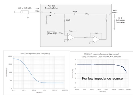
Figure 1. An example of the internal circuit of a rail probe and its impedance profile and transfer function.

With a coax connection, a gain of 1 and high bandwidth, capable of a large DC offset, an active rail probe is ideal for probing a power rail.

Because its input impedance is not constant, a rail probe should NOT be used to probe signals which might come from a driver with a source impedance as large as 1 Ohms or more. The response from such a source would show a distortion of the signal at low frequency due to the frequency dependent voltage divider. With a 1 Ohm source impedance, the voltage divide gain difference between DC and 1 MHz, for example, would be 2%. However, if the source impedance is below 1 Ohms, as is the case for many power rails, there is negligible frequency dependent distortion of the signal.

If you want to measure a power rail, a rail probe is an essential tool for your toolbox. The only downside is that they are sometimes expensive. Enter the economical rail probe.

An alternative method for probing a low-impedance, fast-switching source, with a gain of 1, is the source series termination method, comprising a 50-Ω resistor in series between the DUT and the coaxial-cable connection. The coaxial cable is then connected to the oscilloscope’s analog input set for 1 MΩ termination. An equivalent circuit model and a simple, home-made implementation appears in Figure 2.

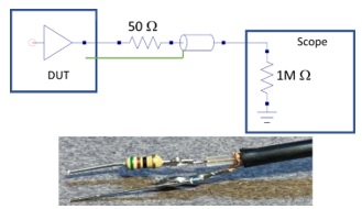
Figure 2: The source series termination method presents
an alternative method of probing low-impedance, fast-switching sources

Avoid 50 Ohm input to the scope when measuring power rails directly

When measuring a high-bandwidth signal line, 50 Ω is the recommended input impedance to the oscilloscope. This prevents the reflection artifacts from the 50 ohm cable between the source impedance of the DUT and the 1 Meg input of the scope.

This is not the case for power rails. There are two important problems created by a 50-Ω input impedance at the oscilloscope when measuring power rails. 

With 50 Ω input impedance to the oscilloscope, the maximum voltage we can probe is 5 V. Higher voltages will dissipate too much power in the scope’s internal 50-Ω resistor and the oscilloscope may suffer damage.

In addition, using 50 Ω for the oscilloscope’s input impedance will introduce a DC load to the DUT. If the DUT is a 3-V source, the 50-Ω load will draw 60 mA. If the DUT can source 100 A, a 60-mA draw from the probe is negligible. But if the DUT is a 100-mA low drop-out (LDO) power source, a 60-mA draw from the probe will dramatically affect the LDO power source’s performance. The act of measuring the rail will affect its performance.

These constraints suggest we should use the 1-MΩ input termination to the scope. The good news is we can measure ±40 V with a negligible DC current draw and offset large DC voltages. The downside is that when probing a low-impedance source with a direct coaxial-cable connection, the oscilloscope’s 1-MΩ input termination will generate large reflections between the cable and low impedance from fast transient edges. This equivalent circuit is shown in Figure 3.

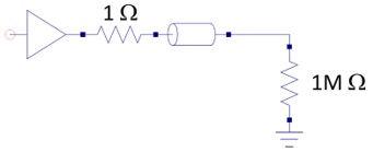
Figure 3: Shown is an equivalent circuit for a direct coaxial-cable connection
to a 1-MΩ oscilloscope input termination

After being launched into the coaxial cable from the low-impedance source, an initial transient signal travels down the coax cable to the oscilloscope’s 1-MΩ input termination. From there, it reflects back to the source. When it again reaches the source’s low impedance, it reflects with a sign change. This reflection makes it to the scope input and pulls the input signal low, then reflects and repeats. The end result is a large ringing artifact measured by the scope.

The answer to this problem: Add a 50-W source series termination to the DUT. As a result, half of the source voltage is initially launched into the coax cable, which reaches the oscilloscope’s 1-MΩ input termination and reflects back. The initial voltage measured by the oscilloscope is 2x the launched voltage, which is exactly the voltage of the source.

When the reflected signal makes its way to the source, it sees the 50-W resistor in series with the low impedance of the source. As long as the source impedance is less than 2 Ω, there is less than 2% reflection, and all the ringing is quickly terminated.

In the example shown in Figure 4, a 5-V switch mode power supply (SMPS) with a 0.1-Ω source impedance switches on with a rise time of a few nanoseconds. It is measured with the oscilloscope set to a 1-MΩ input termination. At left in Figure 4, there is a direct coaxial-cable connection with multiple reflections are clearly evident. At right, the addition of a 50-W source series resistor to the DUT source-terminates the coax cable and prevents multiple reflections. 

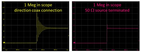
Figure 4: At left: The startup of a 5-V supply when connected to the oscilloscope’s 1-MΩ input termination by a coaxial cable. At right: the results of adding a 50-Ω source series termination to the DUT.

This simple approach of adding a 50-W source series resistance at the end of the coaxial cable is a low-cost alternative to probing power rails at high bandwidth. It is an alternative to using a 10x probe, with the advantage of being a 1x probe that does not attenuate the signal.

Which is better: 10x passive probe or a 1x, rail probe?

What’s wrong with the venerable 10x probe, available in every lab? Why not just use the 10x probe to probe power rails?

In many situations, a 10x probe is the right choice for a power rail. It offers a high impedance to the power rail and able to measure a large DC voltage with a large offset range. And, since 10x probes are shipped with every scope, its effectively free.

A 10x probe or a rail probe can give very similar results when probing low-impedance power rails. Figure 5 shows the measured voltage transient noise on an 18-V SMPS using both probing methods on the same scale. These measurements are DC coupled, with offset applied by the oscilloscope, on a scale of 50 mV/div. This is a very sensitive scale of about 0.25 %/div.

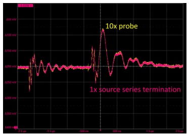
Figure 5: Shown is the transient voltage of an 18-V SMPS measured with
a 10x probe (yellow trace) and with a source series terminated 1x probe (red trace).

In fact, one advantage of a 10x probe is that it can be used for up to ±400 V compared to the ±40-V range of the 1x probe method.

But the 10x probe has two important limitations over a rail probe. Its name is a bit of a misnomer. It is not really a 10x probe. It is a 1/10^th probe. The probe attenuates the signal by a factor of 10. This means that when we try to measure a tip voltage of 100 mV or less, the measured scope voltage is less than 10 mV. This is close enough to the scope noise floor that the signal to noise ratio is reduced. 

Even measuring the 18-V DC level SMPS shown above, the slightly better SNR of the 1x probe is evident. In Figure 6, a 3.3-V SMPS was measured with the same two probes. We clearly see the better SNR of the rail probe.

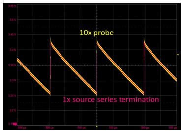
Figure 6: Shown is the transient voltage of a 3.3-V SMPS measured with
a 10x probe (yellow trace) and with a source series terminated 1x probe (red trace).

This distinction defines the condition to decide which type of probing method to use:

If your application is for a voltage level of 10 V DC or higher, the 10x passive probe will be a good choice. It offers higher voltage range with acceptable SNR and is quick, simple, and easy to use. And, everyone has a 10x passive probe.

If your application is for a voltage level of 10 V DC or lower, a 1x passive probe with source series termination will be a better choice. It will provide a better SNR.

Home-made Rail Probe or Active Rail Probe?

The 10x probe and the home-made rail probe are limited by their tip geometry to their sensitivity to RF pick up. If the DUT is in a noisy RF environment, the tip geometry should be as close to a coax as possible. This is one advantage of using an active rail probe with a direct coax connection on the board.

The 10x probe is also limited in bandwidth to about 200 MHz, in the best condition, using a low inductance tip. The tip geometry of the home-made rail probe will similarly limit its bandwidth to about 200 MHz.

To measure transient noise on the power rail with bandwidths higher than about 200 MHz, a coaxial connection to the board with a uniform, controlled impedance through the entire cabling and probe system is essential. This is why an active probe can have a bandwidth as high as 4 GHz.

If your application has a bandwidth above about 200 MHz, the 10x probe and the home-made rail probe suffer from bandwidth limitations. In higher bandwidth applications, consider using an active rail probe that maintains a good 50 Ohm environment from the coaxial connection on the board through the entire length of probe to the scope. But keep in mind the slight gain distortion if the power supply output impedance is greater than about 2 Ohms.

Conclusion

While the 10x passive probe is suitable for many power-rail probing applications, the 50-Ω source series terminated probe is a low-cost, easily homebrewed alternative for the 10x probe, providing better SNR for low-voltage rail applications. However, for high-bandwidth applications, an active voltage-rail probe is the best option.