
We often think that measurements are always correct. After all, it’s how the real world behaves. They are a measure of objective reality. They should not depend on what we think we should get, or what we hope we should get. They are a direct anchor to reality, and we should adjust our theories to conform to the measurements.
This is too simplistic a view of measurements. There is one key missing ingredient which we have to have in order to interpret the measurement: The details on how we performed the measurement and information about the device under test (DUT). You cannot correctly interpret measurements without this key piece of information.
To illustrate the dangers of blindly accepting any measurement, let’s look at the venerable cal signal on the front of every scope. Figure 1 shows an example of the connections to the cal signal on my Teledyne Lecroy 8108A scope. Every Keysight, Tek, and other vendors’ scopes have one of these connections.
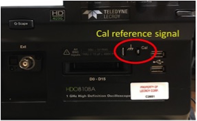
Figure 1. A close up shot of the cal connection on my LeCroy 8108A scope
The signal coming out the cal connection is a square wave. There are four terms that characterize a square wave:
- The repeat frequency
- The peak to peak amplitude
- The duty cycle
- The rise time
Since there is one objective reality of the signal coming off the cal connection, you’d think everyone would measure this signal exactly the same. You’d be wrong. Figure 2 is an example of three measurements, looking at the same cal signal, but getting radically different amplitudes and rise times.
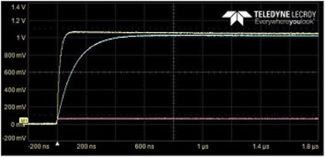
Figure 2. Three different measurements of the cal signal. Which one is correct?
In these examples, the repeat frequency and the duty cycle were exactly the same, but the rise times and the peak-to-peak voltages were measured differently. How can three different measurements of the same signal be so different? Which one is correct? And how would you know?
Who hasn’t measured the cal signal on their scope at some point? What is actually coming out of the source?
There are three important elements we need to consider to unravel this mystery:
- The details of the instrument, in this case, the scope
- The details of the interface from the scope to the source, in this case, the probe
- The details of the source, the actual output peak-to-peak voltage with no load, and its output source impedance and circuit.
As a card-carrying Physicist, I absolutely believe there is an objective reality. The actual voltage waveform present at the cal connection is the same for all observers. But the very act of measuring can change what is actually there. This is one version of the Heisenberg Uncertainty Principle, though not due to a fundamental quantum limit, but to the cost-performance balance we chose when selecting the measurement system.
By understanding the details, we can create a model of reality consistent with all the measurements.
The Details
The scope I used was a Teledyne LeCroy 8108 HDO scope. This has a 1 GHz analog front end bandwidth and samples at 10 Gsamples per second. I am skilled enough in using it that I was sure the same acquisition rates and other settings were used for all the measurements. This is always an important consideration when using modern, high-end scopes since they have so many variables that can be adjusted.
Another important feature to pay attention to when setting up the scope is the input impedance to the amplifier. I used two different values, 50 Ohms and 1 Meg input. The use of 50 Ohms is to prevent reflections in the cable. When using the coaxial cable probe and scope, I have measured signals with rise times at the scope limit of 0.45 nsec 10-90 rise time.
The second piece to this puzzle is the probe. I used three different probes for these measurements. One was a short length of 50 Ohm coax cable with a grabber tip to connected to the cal connector. The second probe I used was a LeCroy PP023 passive probe, the workhorse 10x passive probe, very similar to what is shipped with virtually every scope today. The third probe I used as an old LeCroy PP016 passive 1x and 10 x probe, set for 1x.
Finally, the third piece of the puzzle is the signal source itself. At a minimum, the three most important features of every source you must know are the unloaded voltage output, the source resistance and its other associated circuit elements and the rise time of the signal. If you don’t know these features, you will have no idea how it will behave in any measurement circuit.
By measuring the output voltage level when the impedance loading the signal was very high, and the voltage when loading the signal with a 50 Ohm load, I deduced the unloaded output signal level was 1.02 V and the output impedance was 800 Ohms. It should be noted that this output impedance is very high. This one parameter is the most important term influencing the measured results. Not being aware of the output source impedance contributes to most of the confusion of interpreting signal integrity measurements in general, and these cal signal measurements in particular.
The rise time of the cal signal is a tricky one to measure. It’s important to have confidence that your measurement system of scope and probes has a system measurement bandwidth at least twice as high as the signal’s. Measuring other sources using the coax probe and grabber tips, I’ve measured signal 10%-90% rise times as low as 0.45 nsec, the limit to my 1 GHz scope.
Using a coax probe and grabber tip, I was able to measure a 10% to 90% rise time of 5.0 nsec. I have a high level of confidence my system bandwidth is well above this signal bandwidth, so this is probably a realistic signal rise time.
This means the cal signal is a 1.02 v square wave, coming from an 800 Ohm source with a 5 nsec rise time.
You should now have the pieces of the puzzle to put together the complete picture and unravel the mystery of why I got three different measurements of the same signal. Take a few moments and see if you can figure them out before reading on.
The 50 Ohm Cable Measurement
This was the best I could do to make a controlled impedance, low inductance connection to the clip-on leads of the cal source. A close-up of the probe configuration is shown in Figure 3.

Figure 3. Making a controlled impedance, low inductance connection to the cal connector.
For this measurement, I used a scope input impedance of 50 Ohms. Terminating the 50 Ohm coax into the 50 Ohms of the scope eliminates the reflections from the scope end of the cable. The good news is that any signal which enters the device-end of the coax travels down the cable to the scope and is terminated. Nothing reflects back to the source.
The bad news is we have just attached a 50 Ohm load to the device under test (DUT). When we connect a 50 Ohm load to a source that has a 800 Ohm output impedance, we’ve just created a voltage divider. This means the signal launched into the coax cable is not the 1.02 source voltage but this signal, after a voltage divider, 1.02 V x 50/ (50 + 800) = 60 mV.
This is the signal launched into the coax and travels down to the scope. Once at the scope input, it sees a 50 Ohm resistor and turns into heat with no reflected signal. The amplifier measures the voltage across this 50 Ohm resistor.
Figure 4 shows the measured signal at the scope receiver. It has a 5 nsec rise time and reaches a steady value of 61 mV, exactly as expected. This is the basis of interpreting the output rise time of the source as 5 nsec.

Figure 4. Measured signal at the scope input using 50 Ohm termination and short, 50 Ohm cable with grabber tips.
The 10x Probe
The PP023 probe is similar to the 10x probe shipped with every scope from every vendor. It is designed to be connected to the scope with a 1 Meg termination. A 9 Meg resistor sits at the tip so the signal at the scope, across its 1 Meg resistor, is 1/10 the tip signal. This is the origin of the 10x (really a 1/10th x probe) description.
If you use a 50 Ohm termination at the scope, the voltage divider ratio will be 50 Ohms/9Meg. The resulting signal will be tiny. If the tip voltage is 1 V, the scope voltage will be 5.5uV. That’s why the 8108A scope gives a big warning if you try to use a 50 Ohm termination with the 10x probe.
The probe’s intrinsic bandwidth is 500 MHz. However, this is when measuring a source impedance of 50 Ohms. At high frequency, the input impedance of the probe looks like about a 10 pf capacitor. With a 50 Ohm source driving the probe, and a 1 psec rise time source-signal, the 10-90% rise time would be 2.2 x 50 x 0.01 nF = 1.1 nsec. This is the origin of the 500 MHz bandwidth spec for this probe. I’ve measured shorter rise times when the source impedance was less than 50 Ohms.
When the PP023 probe is connected to the cal source, we measure a rise time of 40 nsec. This is shown in Figure 5. This is much larger than the 5 nsec intrinsic rise time of the source. Why is that?
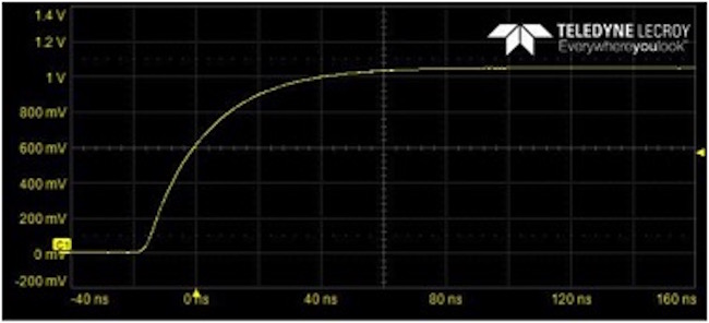
Figure 5. Measured cal source with PP023 10x probe.
With the source impedance of 800 Ohms, we would expect a rise time of 2.2 x 800 x 10 pF = 18 nsec. The measured rise time is still larger than this. Why is that?
If there were an effective 12.5 pF of output capacitance associated with the internal leads to, and connections of, the clips on the front panel of the scope, the effective input capacitance the 800 Ohm source drives would be 12.5 pF + 10 pF = 22.5 pF and the rise time would be 2.2 x 800 x 22.5 pF = 40 nsec. This is consistent with what we measure. Why didn’t we see this in the 50 Ohm cable measurement?
When we connected the 50 Ohm cable across this 12.5 pF capacitance and measured the 5 nsec rise time, the impedance of the 12.5 pF capacitor at the highest frequency of 0.35/5nsec = 70 MHz is 170 Ohms, large compared to the 50 Ohm load shorting it out. This 12.5 pF capacitor was invisible compared to the 50 Ohm load of the cable and we were not sensitive to it.
We see that to explain the observed behavior of this simple cal source there are additional features of the source which play a role influencing the characteristics of the measurement.
The 1x Probe
The older style PP016 probe is designed with a switch on the tip to select the 10x option or the 1x option. With the 1x option selected, the tip is connected directly to the input to the scope, by shorting across the 9 Meg resistor and 10 pF capacitor at the tip.
However, between the tip and the BNC connector that goes to the scope is a very special cable. In ALL 10x probes, the cable is very special. The signal conductor is about 3 mils in diameter, very thin, and composed of a resistive Nichrome alloy. This gives it a series DC resistance of 400 Ohms, which can easily be measured with an Ohmmeter.
In addition, the dielectric is a foamed PTFE which means it has a Dk very close to air, about 1. This combination means the characteristic impedance of the cable is about 200 Ohms and its capacitance per length is about 6 pF/foot. This is compared to 33 pF/foot for RG58, 50 Ohm cable. Figure 6 shows a close-up of the cable cross section.
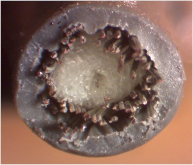
Figure 6. Cross section of the 10x probe cable showing the thin central conductor and foamed dielectric.
The combination of resistive central conductor and high characteristic impedance means the cable is attenuating. The time delay of the cable, based on its 4-ft length, is about 4 nsec. Due to the high characteristic impedance of the cable, the 50 Ohms of the scope is not a good match. When a signal is traveling in the 200 Ohm cable and hits the 50 Ohms of the scope, it will reflect with a reflection coefficient of -75%. This reflection makes its way back to the source and if the source is a low impedance, some fraction will reflect again and head back to the scope.
The round-trip time for a reflection to make it back to the scope is 8 nsec. However, due to the losses, the reflected signal is attenuated. With the cable attenuation, the bandwidth of the cable is reduced. To first order, the RC constant of the cable is about 400 Ohms x 24 pF = 10 nsec. The 10-90% rise time would be on the order of 22 nsec. Reflections at the ends of the cable always happen, but we would never be able to resolve them because they are smeared out over the rise time increase from the cable losses.
We can measure the intrinsic rise time of the cable by measuring a fast signal from a low impedance source. Figure 7 is measured from a 2 nsec rise-time, 20 Ohm source impedance signal using 50 Ohms input to the scope. The measured rise time using this probe is about 18 nsec, very close to our estimate of 22 nsec.
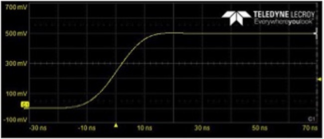
Figure 7. Measured 2 nsec signal with 1x probe and 50 Ohm input.
It’s interesting to note that with this intrinsic cable rise time, the cable bandwidth is 0.35/18 nsec = 20 MHz. This is the bandwidth of the 1x probe on the 50 Ohm scale. This is way below the rated 300 MHz bandwidth for this probe. The bandwidth would be the same even if the source impedance were 1 Ohm. How is this cable able to show a 300 MHz bandwidth in the 10x position?
The secret is in the use of the 9 Meg resistor with a parallel 10 pF capacitor and 1 Meg scope input impedance. When in the 10x setting, the parallel capacitor and resistor at the tip act as a high pass filter to balance the low pass filter of the special attenuating cable. This circuit “equalizes” the cable and gives it a higher bandwidth. This is the same principle used in many high-speed serial links with a Continuous Time Linear Equalizer (CTLE) filter, usually placed at the receiver. The equalizer filter in the 10x probe is built into the tip.
When we connect this 1x probe, without the equalizer, to the 800 Ohm source impedance of the cal signal, and use the 1 Meg input impedance of the scope, we see a peak to peak signal with 1.02 V, as we would expect, but the rise time is measured as about 175 nsec. This is an effective bandwidth of 2 MHz. This is a worthless signal for SI applications. Never use the 1x probe setting.
How did it get so long?
This simple 1x probe is really part of a circuit that has an 800 Ohm source impedance, a 12. 5 pF load at the beginning, a 400 Ohm series, distributed cable resistance and a 24 pF distributed cable capacitance, seeing a 15 pF input capacitance of the scope on the 1 Meg input setting. Just as a rough, first order estimate, the equivalent RC charging time constant for this system is about 2.2 x (800 + 400) x (12.5 pF + 24 pF + 15 pF) = 135 nsec. This is close to the 175 nsec measured 10-90 rise time.
Summary
Making a measurement is easy. Interpreting the results to make sense of what we get can be very subtle. We’ve demonstrated that even the simple cal signal available at the front of every scope in your lab requires detailed information about the scope, the probe and the DUT.
This is always why it is so important to apply rule #9 and analyze every measurement. Don’t accept them blindly.
My buddy, Scott McMorrow, and industry icon, and currently the CTO of Samtec, says, “No one believes a simulation except the person who ran it, but everyone believes a measurement, except the person who took it.”
Maybe now we see value in questioning the details of measurements as well.