For the next generation of high-speed links, edge sampling can be considered an alternative to center sampling in order to relax bandwidth requirements. Architectural decisions depend on the ability to adequately analyze the link. This paper presents a methodology to model and evaluate the performance of both center and edge sampling schemes. Statistical eye analysis is used to determine the performance of the system. Using a cycle accurate bit-true time-domain model for the clock recovery loop, timing impairments are captured and supplied to the statistical eye analysis. As a result, the final statistical eye captures both voltage and timing impairments to better evaluate the system performance. The analysis results demonstrate that depending on the link requirements one of the sampling schemes outperforms the other. The performance crossover point between center and edge sampling under different conditions is presented.
With the demand to transfer larger amounts of digital data in less time, data-rates over single links are increasing. This increase presents a growing challenge to reliable detection of data once it travels through lossy transmission media. We need faster transceiver circuits to condition and detect the signal that has suffered from attenuation and dispersion of the channel. While faster fabrication technologies can offer a solution, they usually fall short in keeping up with the growing data rates. As a result, the ultimate solution so far has been a combination of efforts including faster technologies, more efficient modulation schemes, error correction techniques, as well as innovations in the transceiver architectural and circuit designs [1],[2],[3].
The industry’s migration from binary non-return to zero (NRZ) to pulse amplitude modulation (PAM) was an attempt to answer the bandwidth challenge of the link from a modulation efficiency improvement point of view [4]. One aspect of detection is to decide on the sampling phase of the signal. It is the goal of this study to statistically analyze the effect of sampling phase on relaxing the challenging requirement of the transceiver architecture and its circuit implementation and eventually quantify the link performance. This can allow architectural choices to be made earlier in the design phase without having to run potentially long and cumbersome simulations.
Center Sampling
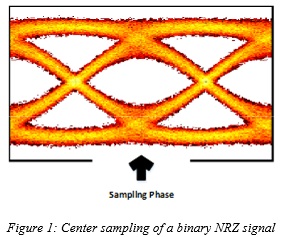
Achieving the required bandwidth of the receiver front-end circuitry has proven to be the most challenging obstacle to conditioning the received signal for detection. Traditionally, signal conditioning has consisted of equalizing the signal by employing a combination of several techniques such as feed-forward equalization (FFE), continuous-time linear equalization (CTLE), and decision-feedback equalization (DFE) in an effort to open up the eye diagram of the signal so that the effect of inter-symbol interference (ISI) on the sampled values is minimized (while other side effects such as noise enhancement are adequately controlled). The usual historical approach is to sample the signal at its highest peak to maximize the signal energy which corresponds to locking the sampling phase of the clock and data recovery (CDR) unit at the center point of the eye diagram (center-locked clock phase) [5],[6]. This approach is referred to as center sampling in this paper and is illustrated in Figure 1 for a binary NRZ signaling scheme.
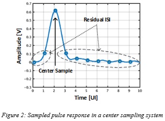
The sampled pulse response corresponding to a typical center sampling system is shown in Figure 2, where the CDR has attempted to locate its sampling clock phase near to the peak point of the equalized pulse. The pre and post cursors (ISI samples) are spaced from the center sample by multiples of a baud-rate unit interval (UI).
Edge Sampling
The exemplary pulse response of Figure 2 arguably illustrates an under-equalization scenario mainly due to the noticeable presence of the first pre and post residual ISI terms, which on their own account for almost 30% of the eye closure in this example. Depending on other impairments, to achieve a better bit-error rate (BER) performance, it might be beneficial to increase the amount of equalization.
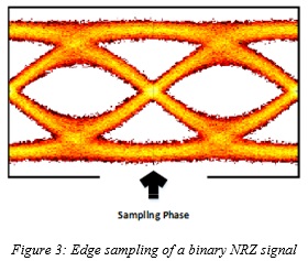
Optimizing system performance requires designing the transceiver for an optimized utilization of equalization techniques and results in a compromised level of equalization due to the inclusion of other considerations. For example, including power consumption of the transceiver as a part of optimization usually prohibits extensive use of FFE and DFE, particularly at higher data-rates. In these cases, and as one possible alternative, one may consider changing the sampling point of the eye diagram from its center position to edge for reasons that will be explained here. This approach, namely edge sampling in this paper, is depicted in Figure 3 for a binary NRZ eye plot.
The pulse response sampled by a clock phase that locks to the threshold crossings of the signal (edge-locked clock phase) is illustrated in Figure 4 for the same pulse response of Figure 2.
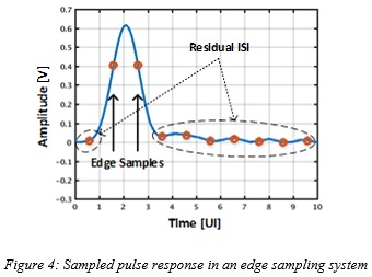
The potential advantage of edge sampling can be more explicitly understood by noticing the reduced amount of residual ISI in the sampled values shown by Figure 4, compared to center sampling, shown by Figure 2. Note that this reduction in ISI is achieved without any increase in the gain and bandwidth of the transceiver circuitry and particularly the CTLE, although one might argue that the edge sample values are now reduced compared to the center sample, resulting in a reduced signal-to-noise ratio (SNR).
However, depending on the contribution of different impairments, the overall SNR can indeed be higher if all of the impairment components, including ISI, are included in calculating the overall noise. This is somewhat illustrated in the eye diagrams used in Figure 1 and Figure 3 when one compares the opening of the center eye in Figure 1 with the opening of the edge eye in Figure 3 and notices that, depending on the impairments, the decision may not be trivial and requires a deeper analysis.
Furthermore, if the detection method is allowed to extend beyond the traditional symbol-by-symbol technique, edge sampling can enjoy an additional leverage offered by a sequence detection technique, making the decision even more non-trivial. Using more exotic detection techniques would have area and power implications that can be incorporated in the overall system architecture optimization process. These arguments suggest that a crossover point in the BER performances of the center sampling and edge sampling systems exists, which if falls within the window of operation in a practical situation, can be essential in deciding which approach outperforms.
Edge Sampling and Partial-Response Signaling
In a typical transceiver design, the equalized pulse response is almost symmetric around the center sample so that the edge samples are equal and spaced at ±0.5UI from the center sample. This results in an edge sampling pulse that can be represented by a partially-equalized response [7] and resembles a duobinary partial-response signaling (PRS) scheme described by a 1 + D coding polynomial ( D represents 1UI delay) [8].
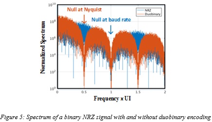
Although demonstrated by the above sampled pulse examples, the lower bandwidth requirement of the edge sampling method compared to center sampling can be better understood by the resemblance between edge sampling and duobinary systems. The coding polynomial of the duobinary system results in an additional  signal transfer function, which creates a spectral null in the signal spectrum at the Nyquist frequency.
It is general practice that in a center sampling system the bandwidth of the transceiver circuitry should at least extend to the Nyquist frequency located at half of the baud-rate, where there is a null at the spectrum of the signal. However, introduction of the spectral null at the Nyquist frequency by the duobinary transfer function suggests that the required system bandwidth can now be reduced by an almost factor of two to half of the Nyquist frequency. This is illustrated in Figure 5, where the spectrums of a binary NRZ signal with and without duobinary encoding are plotted.
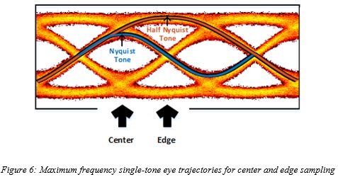
This bandwidth reduction in the signal manifests itself in the time domain by observing the maximum frequency single-tone trajectories through the eye traces. This is depicted in Figure 6, where these trajectories are highlights for the center and edge sampling scenarios.
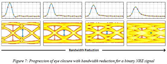
From the above explanations, it becomes evident that if for any reason, such as circuit design challenges in a specific fabrication technology or excessive noise enhancement due to high bandwidth, it is preferable to reduce the bandwidth below the Nyquist frequency, it affects the center eye opening more quickly than the edge eye opening due to the dominance of residual ISI. For example, at a bandwidth close to half the Nyquist frequency, while the center eye is most likely completely closed and center sampling is no-longer viable, the edge eye can still be open and the link may continue to perform if edge sampling is employed. Equivalently, for a given upper limit of bandwidth, as data-rates increase there may be a point at which while the center samples cannot provide reliable detection, edge samples may still be able to do so.
Figure 7 sketches an example of the progression of center and edge eye closures as the bandwidth of the transceiver is reduced. As can be seen from this figure, while both eye openings shrink with bandwidth reduction, it does so more rapidly for the center eye, confirming existence of a crossover point.
Detection of Edge Samples
The detection process (which involves converting the equalized signal to best estimates of the transmitted data symbols) also affects the BER performance of the transceiver. Assuming adequate equalization, while detection of center samples is simply slicing the signal to its original data levels, detection of edge samples involves an additional step which is removing the remaining ISI from the partially-equalized edge samples.
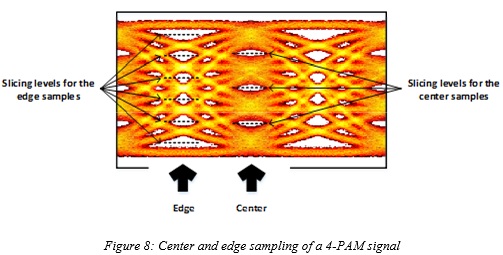
One straight-forward approach is to use a 1-tap DFE, which essentially functions as a slicer with a threshold level set by the previous decision. For a binary NRZ, this would mean slicing the upper or lower segment of the edge eye at a level that depends on the outcome of the previous binary decision. In a more general M-level PAM (M-PAM) scheme, there will be 2M-1 distinct levels for the partially-equalized edge samples and 2M-2 stacked edge eye openings and slicing levels for the DFE.
Figure 8 shows the center and edge sampling of an equalized 4-PAM signal. Three slicing levels for simple detection of center samples and six slicing levels for the DFE detection of edge samples are shown in this figure. Note that in both cases the detection results in one of the four levels of the 4-PAM signal.
DFE detection of edge samples is prone to error propagation. This makes direct comparison between edge and center sampling on the basis of eye opening inaccurate, unless either the effect of error propagation is included during the comparison or error propagation is avoided altogether. To address error propagation in practical applications where edge sampling is to be employed, the transmitted symbols are often pre-coded in the transmitter. The process of pre-coding is outside the scope of this work, but in summary involves moving the DFE from the receiver to the transmitter and using modulo-M subtraction instead of linear summation within the DFE loop. As a result, the detection of edge samples changes from a memory-based DFE operation to a memory-less modulo-M slicing operation [9]. This makes comparing the error performances of center and edge sampling schemes based on their corresponding eye openings a fair and accurate comparison.
The detection techniques of the edge samples discussed so far use a symbol-by-symbol approach. The existence of the 1 + D coding polynomial in the edge samples introduces redundancy in the sequence of signal levels that will not be exploited by symbol-by-symbol detection. Maximum-likelihood sequence detection (MLSD) is an alternative detection approach that takes advantage of this coding redundancy to improve the error performance of the detector [10]. However, this improvement comes at a price (e.g. power, area, and latency) that may not be feasible for all applications. The description of a MLSD detector is beyond the scope of this work, but it has been shown that the application of it to the duobinary case can result in almost 3dB improvement in the SNR and significant reduction in BER [11].
Statistical Eye Analysis
Regardless of the detection technique used to extract the data from the edge samples, and as long as its impact on the performance can be quantified and included in the BER calculations, eye opening calculation based on statistical analysis can still be used to assess the performance of edge sampling and compare it with center sampling. Without any bias towards either one of these sampling schemes or detection techniques, it is the goal of this work to use the analysis to quantify the crossover point between the two techniques in the presence of as many critical impairments as possible. Furthermore, the analysis also provides sensitivity data which can assist with the architectural decisions of the transceiver for practical applications.
This section will outline a methodology to determine the optimal sampling technique given a set of constraints for the link. In the proposed approach, it is assumed that the data-rate is fixed and we would like to increase the channel loss as much as possible. There are restrictions placed on the CTLE bandwidth that is achievable based on a fixed technology node. While this analysis is choosing to keep the data-rate constant, the methodology would similarly apply for attempting to increase the data-rate while keeping the channel profile constant, or a combination thereof.
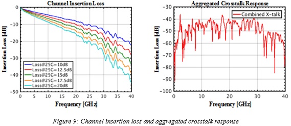
The channel insertion loss and aggregated crosstalk response for an exemplary link are shown in Figure 9. The goal of the analysis is to find the range of channel losses for which edge sampling outperforms center sampling. The insertion loss at which edge sampling outperforms center sampling will be referred to as the crossover point.
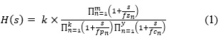
We will be setting some constraints on the design of the analog circuits, mainly the CTLE, to mimic the limitations posed by a certain technology. We assume that the CTLE transfer function can be characterized in the format shown in Equation (1):
 (1)
(1)
The CTLE has a broadband gain of K , m adjustable zeros, k adjustable poles, and y fixed poles. The fixed poles are the parasitic poles of the CTLE which cannot be pushed higher due to technology limits. The exact values of these limits need to be obtained after some technology investigation. For the remainder of the analysis it is assumed that  In a
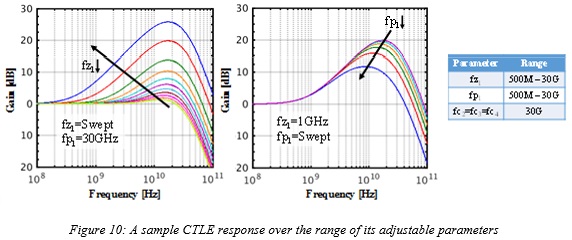
In a  CMOS technology, after some transistor level simulations it is determined that for a reasonable power the parasitic pole frequencies cannot be increased beyond 30GHz . As a result, for the initial analysis, a parasitic pole frequency of 30GHz is used. However, later in the analysis that number is also varied to see the effect. A sample CTLE gain curve over the range of its adjustable parameters is shown in Figure 10.
The next step in the methodology is to determine a metric to be able to fairly compare different modulation schemes. The performance of the system needs to be verified under different channel losses and modulation schemes. To perform the analysis, a statistical tool is used to model the eye opening prior to the slicing latches under different operating conditions.
A sample statistical eye diagram for both center and edge sampling is shown in Figure 11. From the statistical tool, the eye opening can be obtained at different BERs. For our analysis, the link requires a 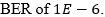 Several parameters of the eye opening can be used as a metric for overall link performance. Although the vertical eye opening at the sampling point is frequently used as the metric, the same analysis can easily be applied if horizontal eye opening or other metrics such as eye opening area is used as the metric. The calculation of the eye opening depends on the sampling point. In later sections, different clocking architectures for both center and edge sampling schemes along with how the sampling point is determined will be discussed.
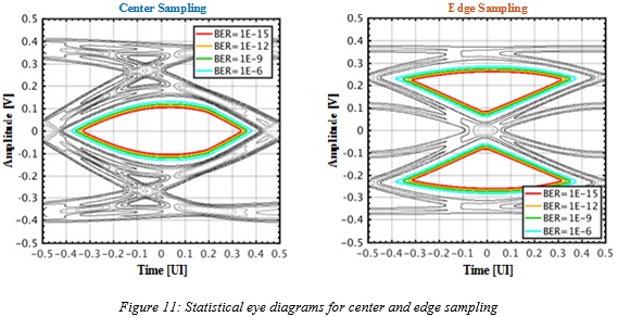
In each of the statistical simulations that are shown in Figure 11, several different impairments are included to help obtain an accurate representation of the performance. Firstly, the effect of the ISI from the combined channel plus CTLE response is captured from the simulated pulse response of the complete channel. Secondly, the effect of crosstalk from adjacent links is included. Thirdly, the effect of nonlinearity in the CTLE response is included to account for any supply voltage limitations of the technology process in the form of signal compression. Fourthly, thermal noise is added in the model as a Gaussian random variable.
The thermal noise is assumed to have a constant power spectral density at the input of the CTLE which is then shaped by the CTLE response. The ultimate eye opening in the presence of all the different impairments is used to judge the performance of a system at a given data-rate for center and edge sampling schemes. As mentioned in the previous section, the effect of some other implementation options, such as encoding and detection technique, can be factored in terms of their impact on the BER or effective signal strength.
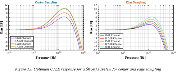
For each condition being simulated (specific channel loss and center/edge sampling), the CTLE is optimized within the outlined constraints in Figure 10. All the CTLE parameters (adjustable poles/zeros) are chosen to give the maximum vertical opening at the required 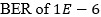 after all the voltage impairments are included. Figure 12 shows the optimal CTLE response for a data-rate of
  for both center and edge sampling for different channel losses. As can be seen, the total amount of required equalization is lower for the edge sampling. In this example, the center sampling cannot achieve an open eye for a channel with the given CTLE constraints and as a result an optimal CTLE curve is not provided for that loss.